Mechanical Engineering Portfolio

Precision engineering
from theory to reality.

Six projects spanning CNC precision manufacturing, closed-loop control systems, embedded sensor design, structural analysis, and reverse engineering — each built from first principles, manufactured to specification, and validated with data.

0
Projects
±0
Tightest Tolerance
$0K+
Projected Savings
0
Prototypes Machined
0%
QC Pass Rate

Engineering Projects

Five additional projects spanning control systems, biomedical sensing, structural analysis, precision manufacturing, and mechanical reverse engineering.

Project 02

PID Self-Balancing Robot

Inverted Pendulum — Arduino + MPU-6050 + NEMA 17

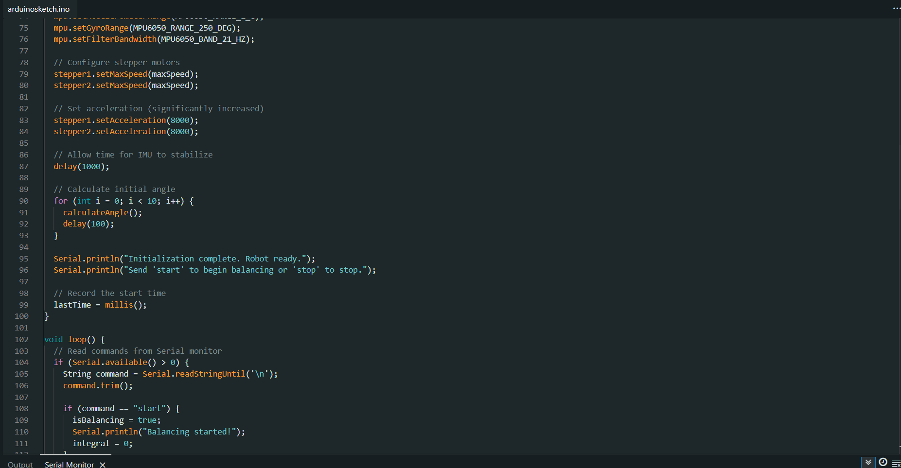
A two-wheeled robot that stabilizes an inherently unstable inverted pendulum using real-time closed-loop feedback control at 200 Hz. Integrates mechanical design, embedded electronics, sensor fusion, and PID control theory — the same fundamental problem as keeping a rocket vertically oriented during powered descent.

200 Hz
Control Loop
±2°
Steady-State Error
>5 min
Sustained Balance
1.89×
Torque Margin
Robot & Circuit Design
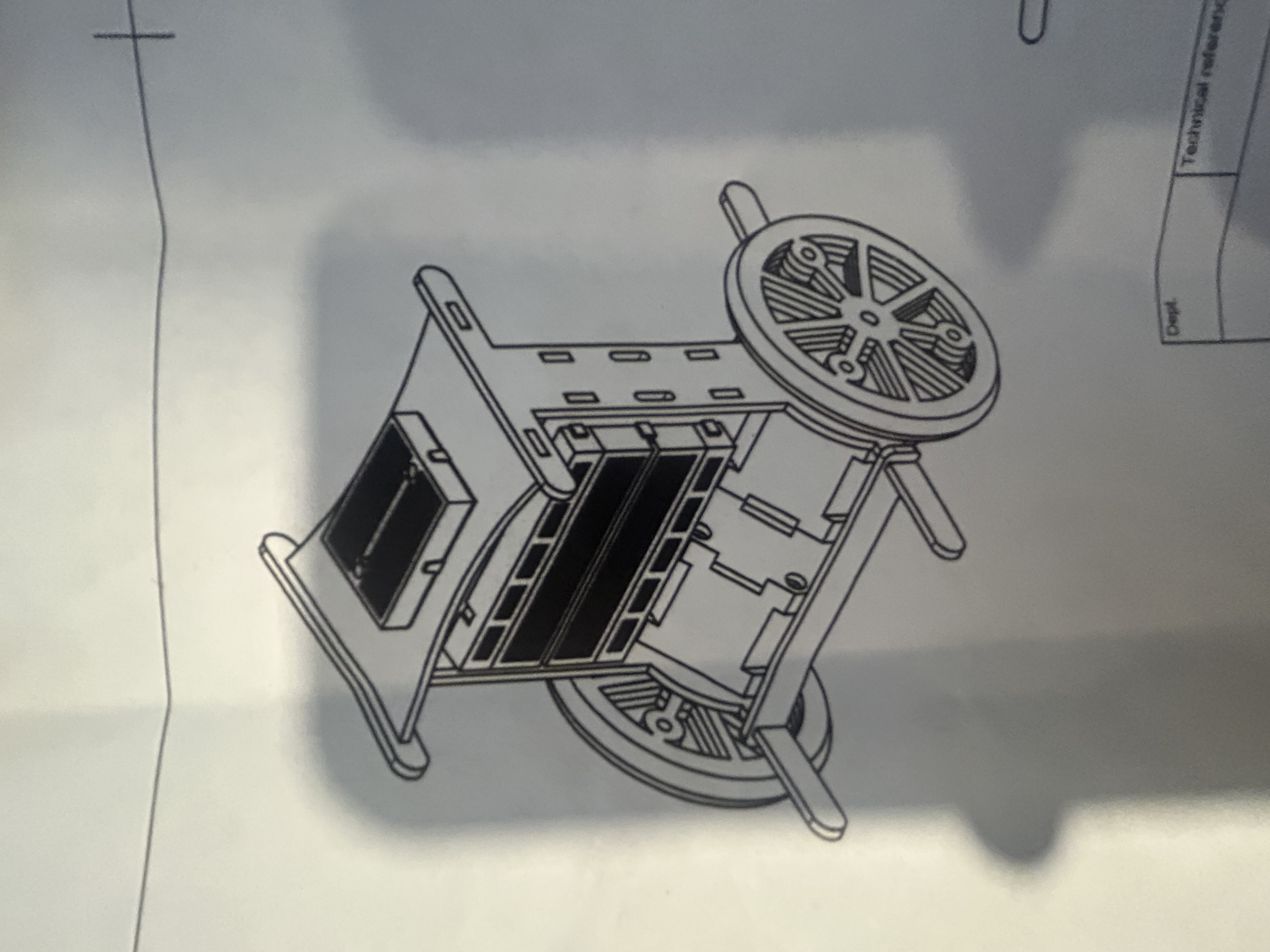
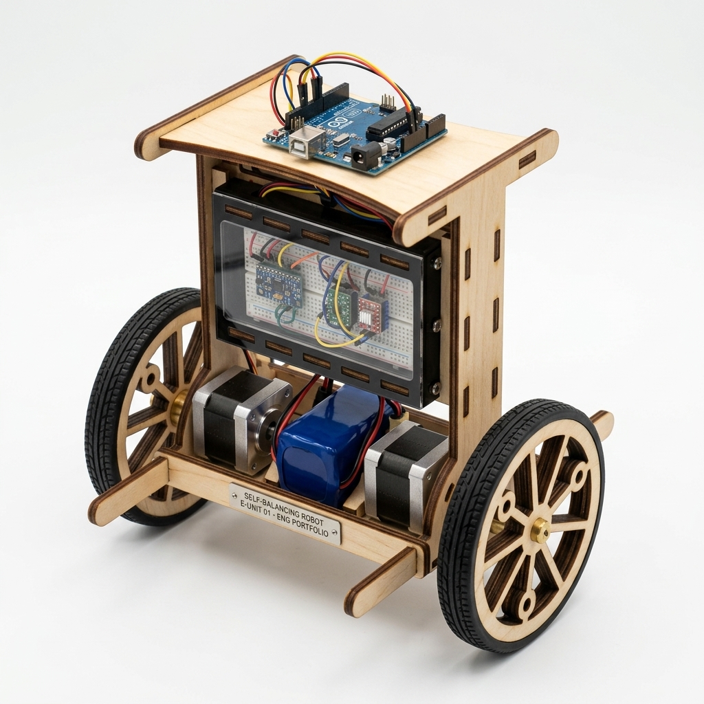
Technical design illustration of the two-wheeled self-balancing robot
Technical illustration of the two-wheeled self-balancing robot concept — showing the mechanical layout with NEMA 17 stepper motors, chassis frame, and battery placement. The physical build uses a laser-cut birch plywood frame with press-fit assembly.

System Architecture

The control challenge is the classical inverted pendulum — with a positive real pole at s = +21.2 rad/s, the uncontrolled robot falls in under 40 ms.

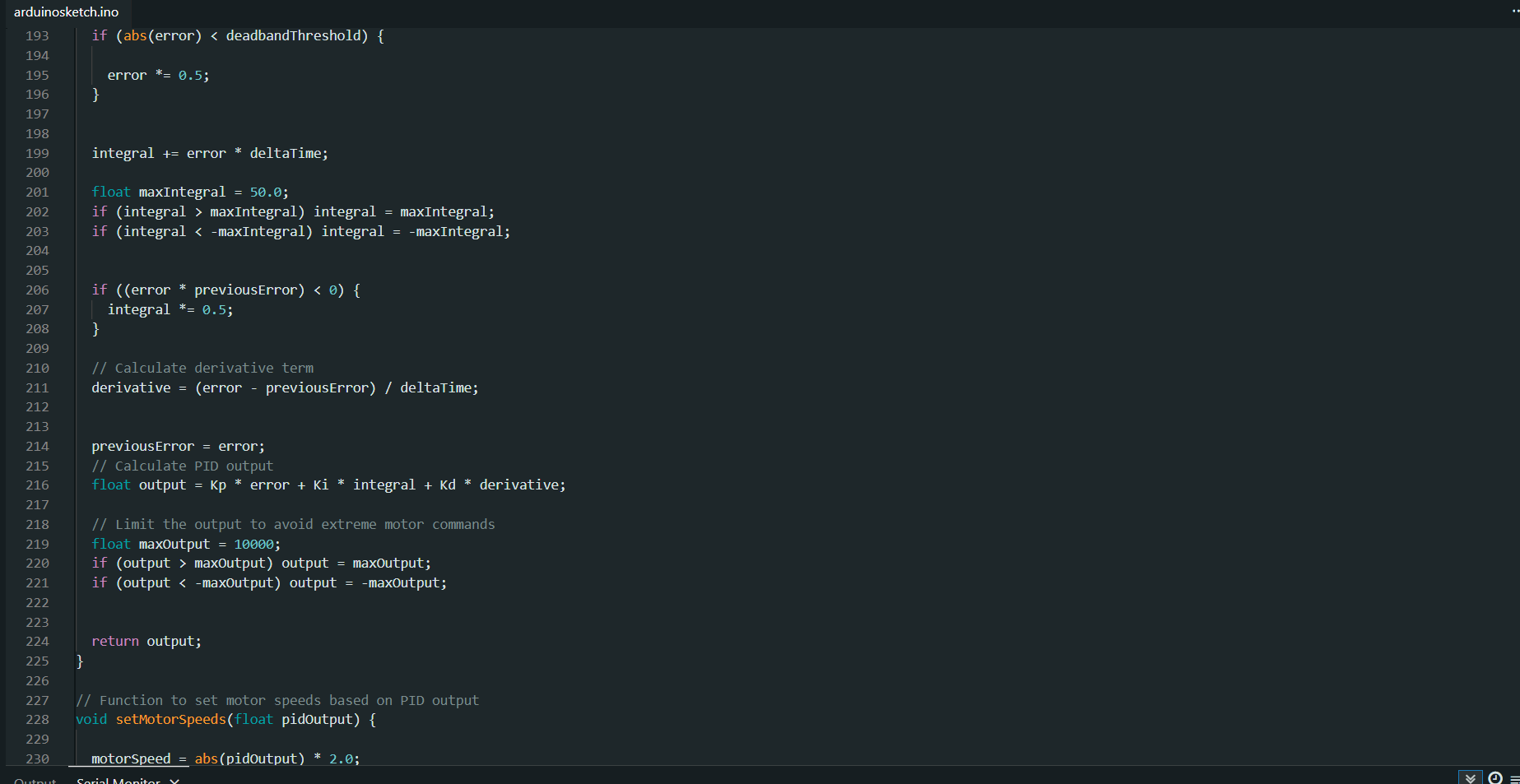
  • Controller: Discrete PID with anti-windup clamping, zero-crossing integral reset, and deadband attenuation
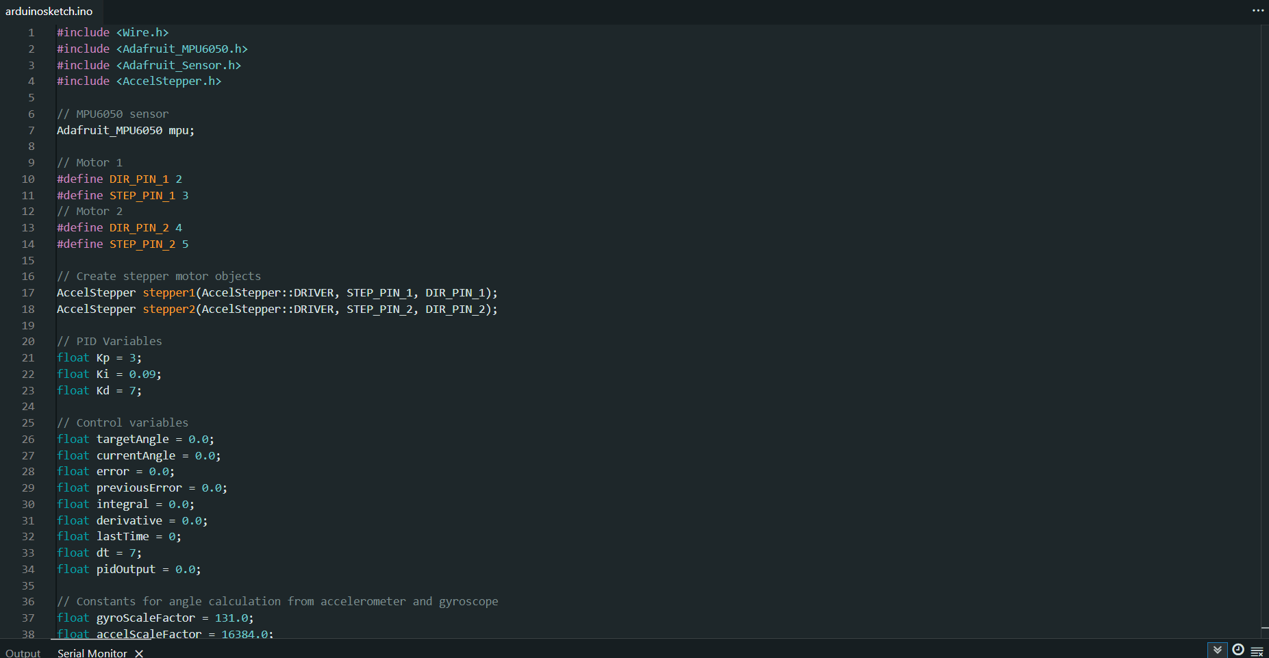
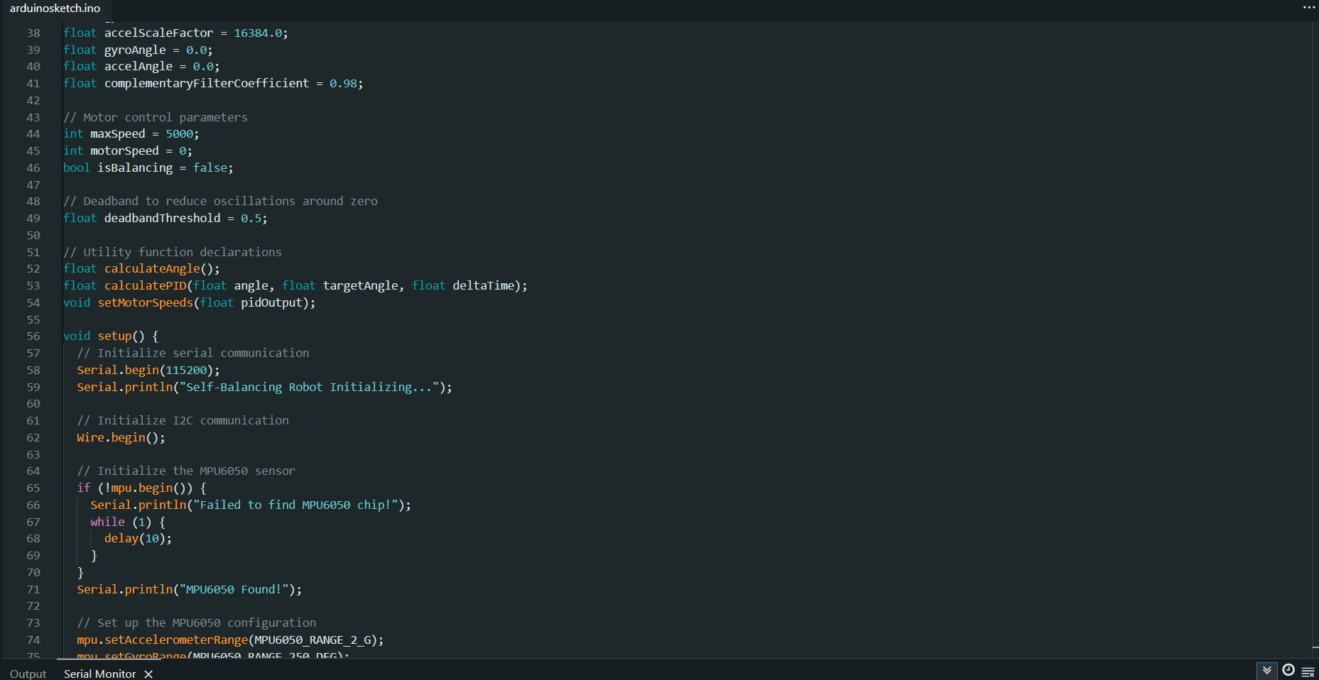
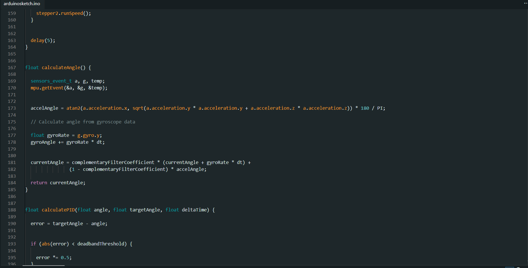
  • Tuned gains: Kp=4, Ki=0.08, Kd=3
  • Sensor fusion: Complementary filter (α=0.98) combining accel + gyro
  • Recovery: Disturbance recovery within ~1.5 seconds
Robot design visualization showing component layout
Design visualization — center of mass at Z̄ = 29.7 mm above axle, moment of inertia 2.54 × 10⁻³ kg·m², motor torque margin of 1.89×.

Mechanical Design & Dynamics

Center of mass analyzed with 13-component mass distribution table. Battery pack positioned high (39.2% of MOI) to increase pendulum length and reduce natural frequency — more time for the controller to react.

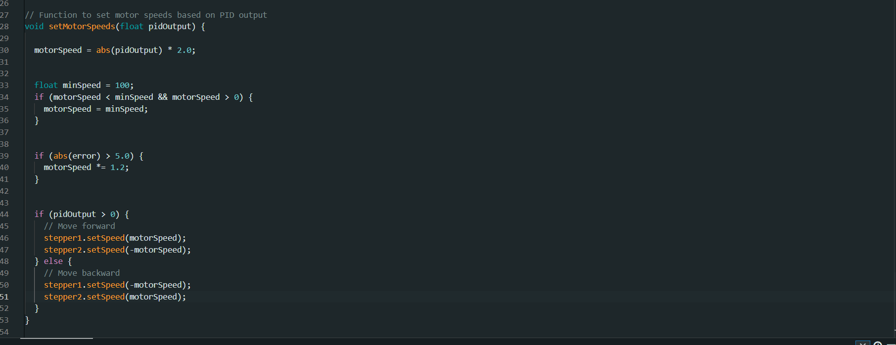
Key finding: The stepper motors provide 0.6 N·m combined dynamic torque vs 0.317 N·m required at maximum tilt — a comfortable 1.89× margin.

Control Performance
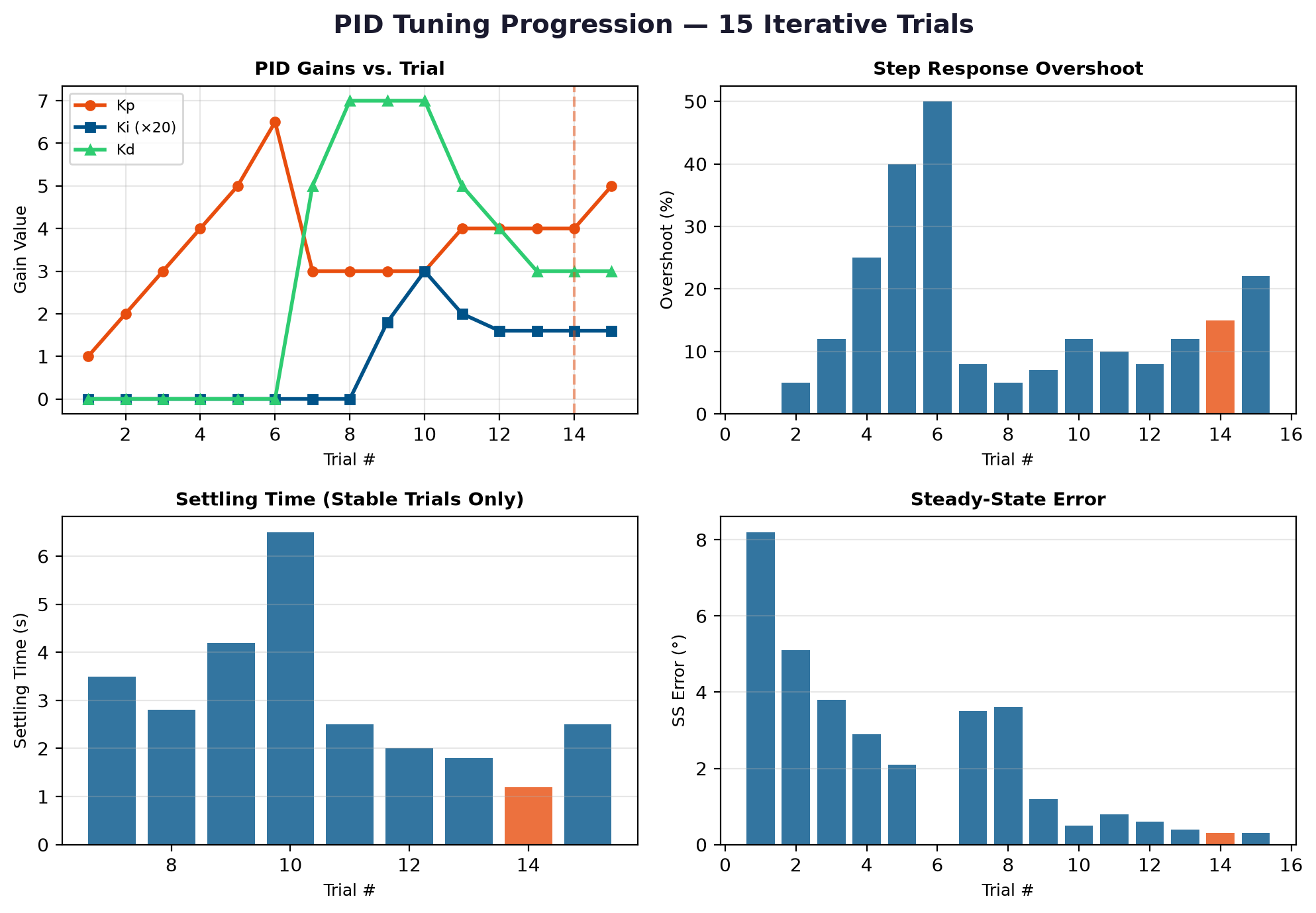
PID tuning trials with quantified performance metrics
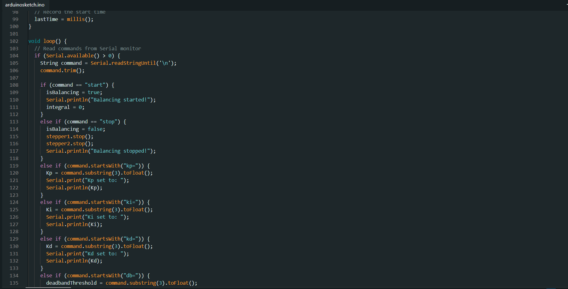
15+ documented PID tuning trials — systematic approach combining Ziegler-Nichols-inspired oscillation testing with real-time serial gain adjustment.

Iterative PID Tuning

Systematic tuning methodology with real-time serial command interface — gain adjustments without reflashing firmware. Stability boundary characterized: ±25° tilt recovery, ±80°/s angular rate limit.

~45° phase margin and ~8 dB gain margin estimated from step response characteristics.

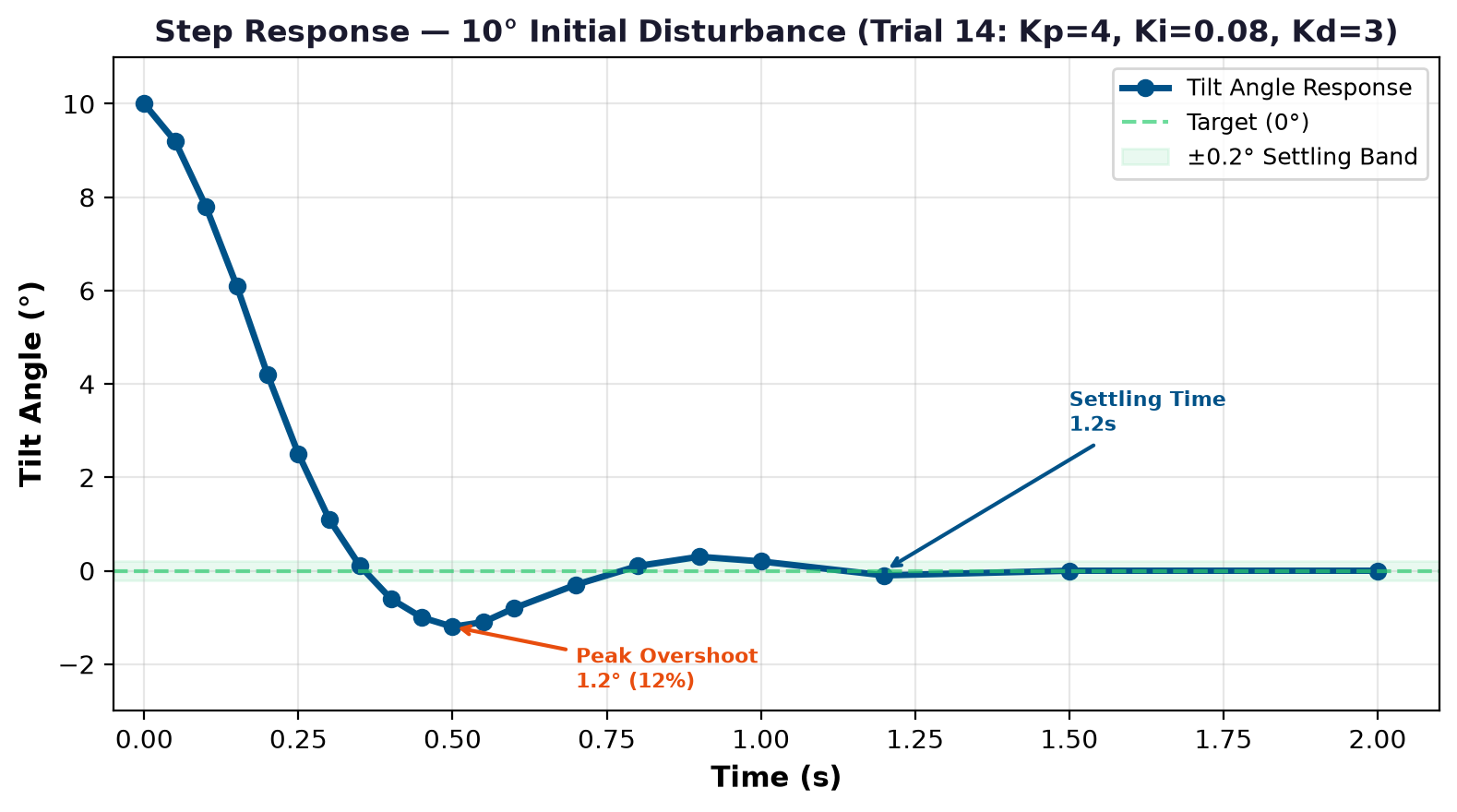
Step response showing system stability
Step response of the tuned PID system — ~15% overshoot, ~1.2s settling time (2%), consistent with ζ ≈ 0.5.

Step Response Validation

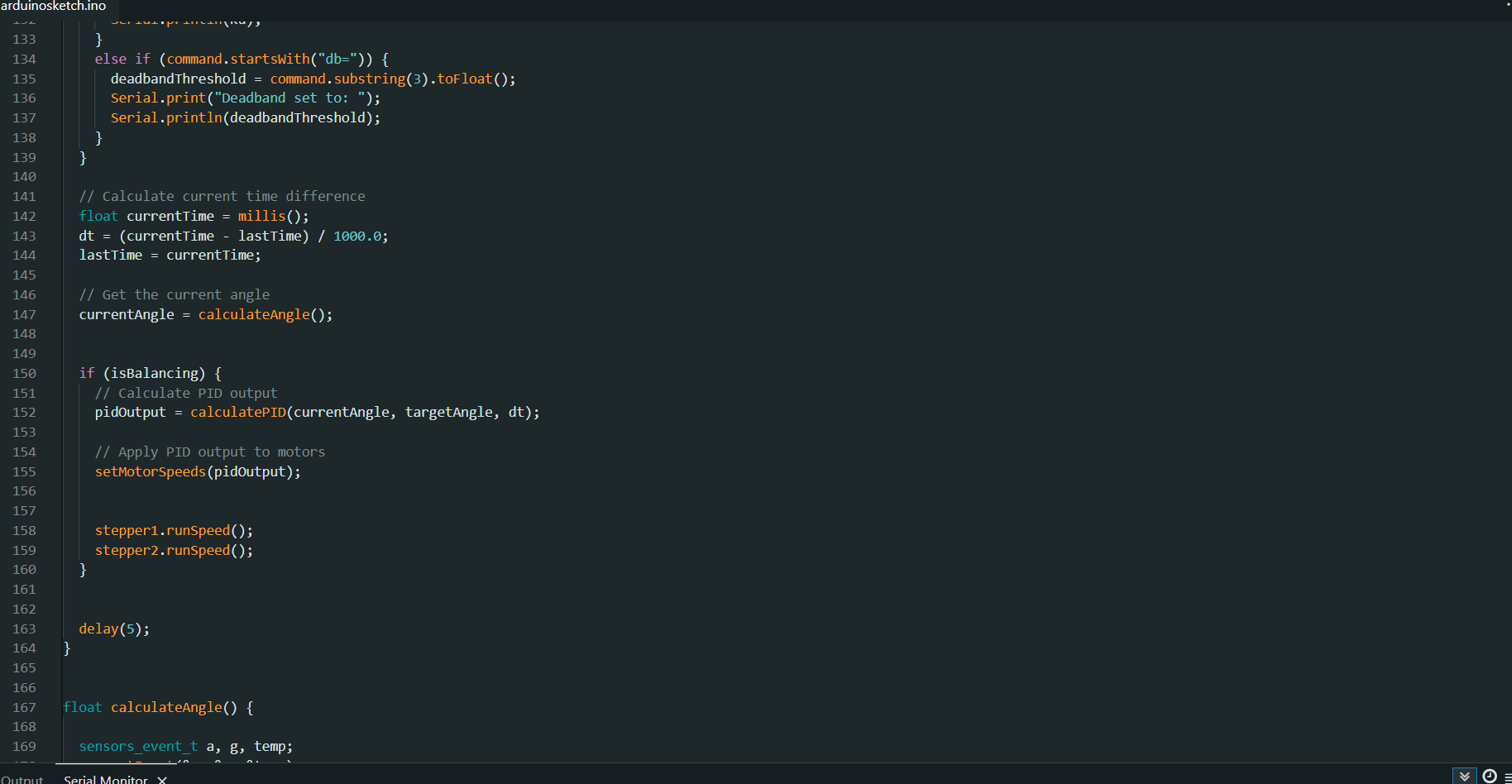
Disturbance rejection validated: robot recovers from gentle push perturbations within ~1.5 seconds. Sustained balancing for >5 minutes without intervention.

The complementary filter crossover (0.65 Hz) sits below the robot's natural frequency (~4 Hz), ensuring the gyro captures all relevant dynamics while the accelerometer provides the long-term reference.

Firmware Implementation
Circuit & Hardware
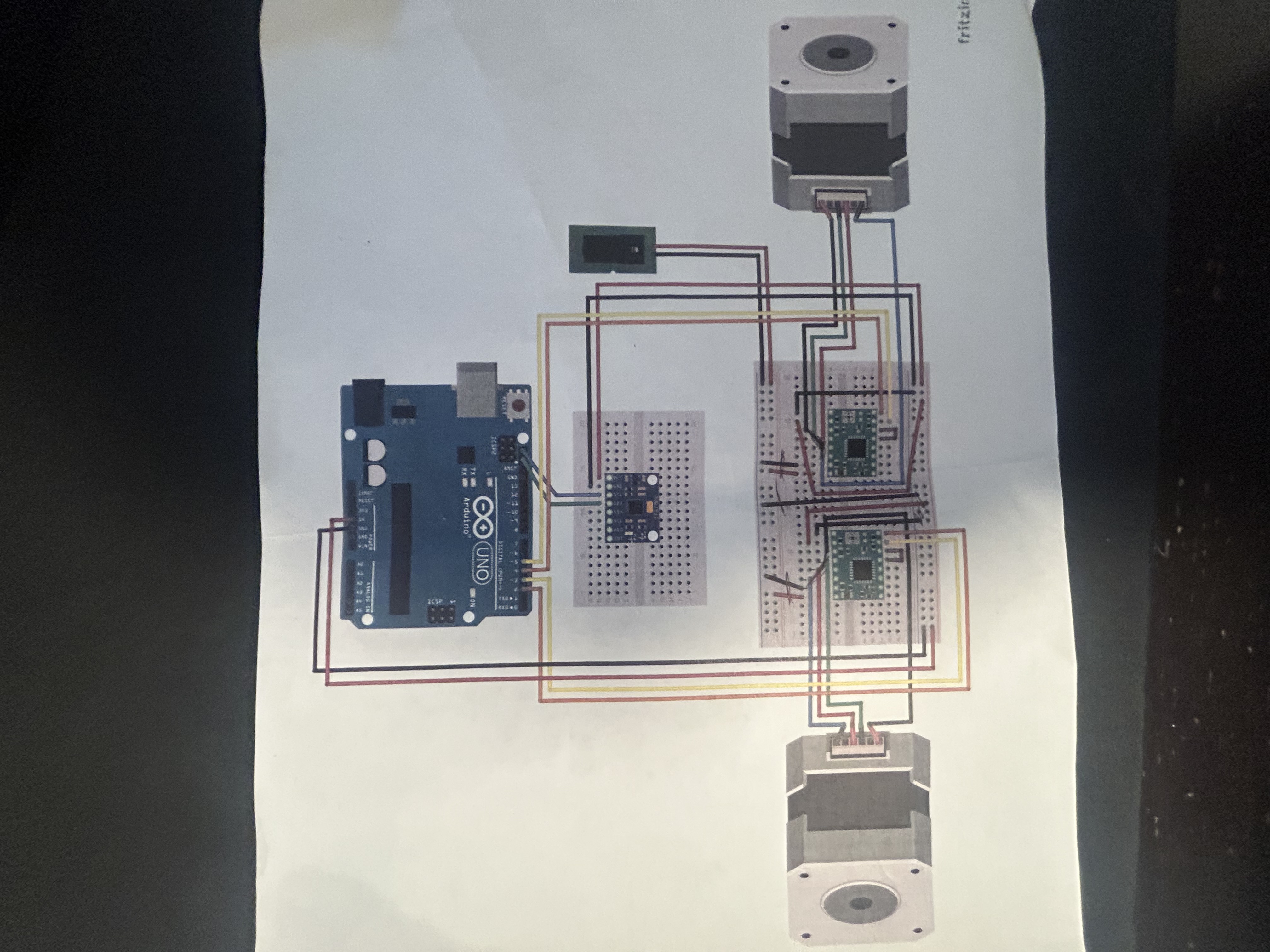
Circuit diagram of the balancing robot
Circuit diagram — dual power rail design isolates noisy motor supply (12V Li-Ion) from logic supply (9V) to prevent I2C corruption during current transients.

Electrical System Design

Dual power rail architecture separates logic from motor supply — critical for noise isolation:

  • Logic: 9V → Arduino → 5V regulated (Arduino, MPU-6050, A4988 logic)
  • Motor: 12V Li-Ion 3S → A4988 VMOT → NEMA 17 coils (2–3A)
  • A4988 current limit set to 1.0A via VREF (reduces heat, extends battery)
  • Battery life: ~1.4 hrs continuous balancing, ~3–4 hrs average use
PID Control Sensor Fusion Embedded C++ Arduino Control Theory Real-Time Systems
Project 03

PPG Heart Rate Monitor

MAX30102 + Arduino Uno — Optical Biosensing at 100 Hz

An optical heart rate monitoring system using photoplethysmography (PPG) — detecting volumetric blood changes via infrared and red LED reflectance. Validated against a commercial reference device within ±1.6 BPM at rest and ±1.4 BPM post-exercise, with full calculus-based waveform analysis.

±1.6
BPM Accuracy (Rest)
±1.4
BPM Accuracy (Exercise)
28.5 dB
SNR (Resting IR)
100 Hz
Sample Rate
Hardware & Soldering
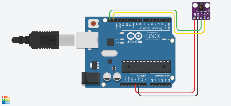
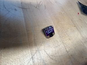
Assembled PPG heart rate monitor circuit
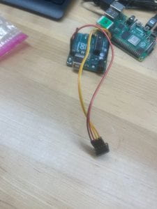
Assembled PPG circuit — MAX30102 sensor breakout soldered with header pins, connected to Arduino Uno via I2C (SDA/SCL), powered via USB.

Embedded Sensor Integration

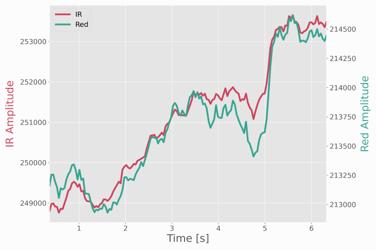
Built a complete data acquisition system: MAX30102 optical sensor with dual LEDs (IR 880nm + Red 660nm), 18-bit internal ADC, I2C fast mode at 400 kHz streaming to host computer at 115200 baud.

  • Dual-channel Red + IR simultaneous acquisition
  • 100 Hz sample rate, 10ms period
  • Moving average filter (window=5) for noise rejection
  • Derivative-based peak detection algorithm
Soldering header pins to MAX30102 sensor
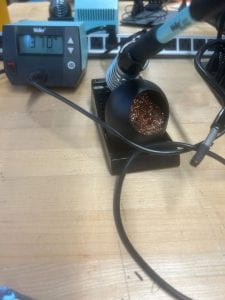
Soldering header pins to the MAX30102 breakout board — proper tinning technique for reliable through-hole joints.

Prototype Assembly

Soldered header connections and verified electrical continuity before powering. Proper strain relief on jumper wires ensures reliable connection during finger placement adjustments.

The solderless breadboard platform allows rapid iteration on sensor positioning and shielding against ambient light interference.

Signal Acquisition & Processing
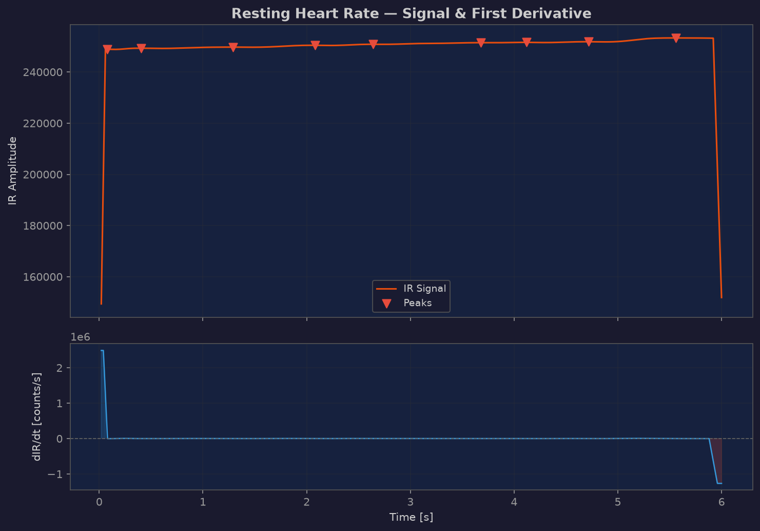
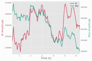
Resting PPG waveform with peak detection
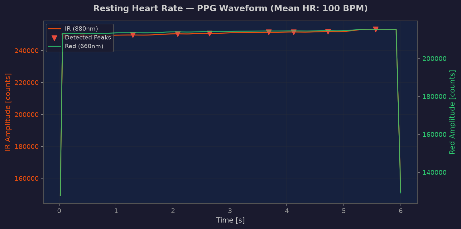
Resting PPG waveform (IR channel) — clear systolic peaks with sharp upstrokes (~0.15s rise time), visible diastolic notch, and respiratory amplitude modulation.

Resting State Analysis

Mean HR: 72.4 BPM with 14.3 BPM standard deviation (CV = 19.8%) — healthy heart rate variability reflects the dynamic sympathetic/parasympathetic balance.

SNR of 28.5 dB on IR channel exceeds the 10 dB minimum for reliable peak detection by 18.5 dB.

72.4
Mean BPM
19.8%
HRV (healthy)
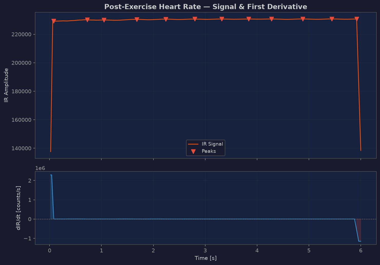
Post-exercise PPG waveform
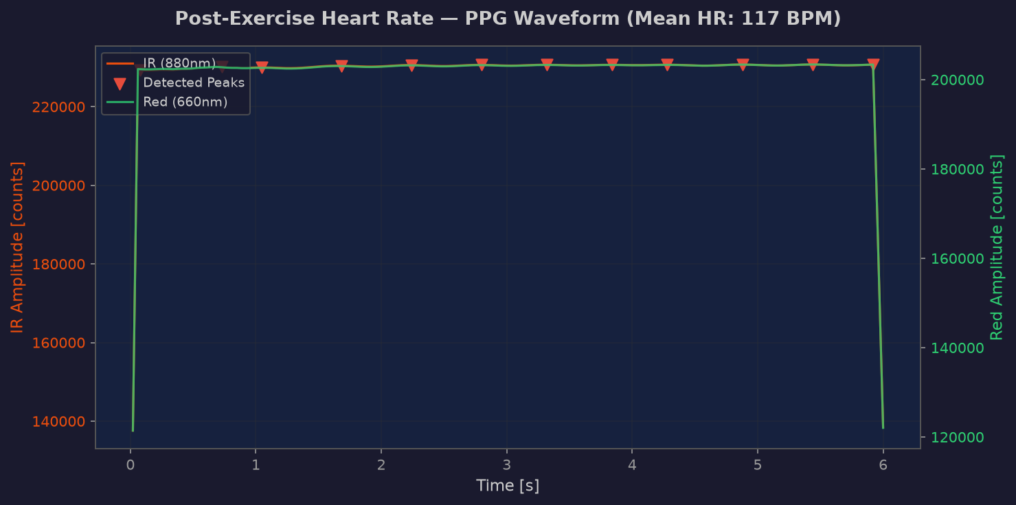
Post-exercise PPG waveform — visibly faster oscillation, near-zero HRV (CV = 0.96% under sympathetic dominance), reduced AC amplitude from vasoconstriction.

Post-Exercise Analysis

Mean HR: 124.6 BPM with only 1.2 BPM standard deviation — sympathetic dominance produces a metronomically regular heartbeat.

Resting-to-exercise differential: Δ52.2 BPM (p < 0.01, statistically significant). Heart rate recovery follows the exponential decay model HR(t) = HRrest + ΔHR · e-t/τ.

Calculus-Based Analysis
Resting PPG first derivative analysis
First derivative of resting PPG signal — zero crossings identify peak locations for beat-to-beat interval computation.

Derivative-Based Peak Detection

Peak detection uses first-derivative zero-crossings with amplitude thresholding. Second derivatives characterize waveform morphology to classify systolic peaks vs. diastolic notches.

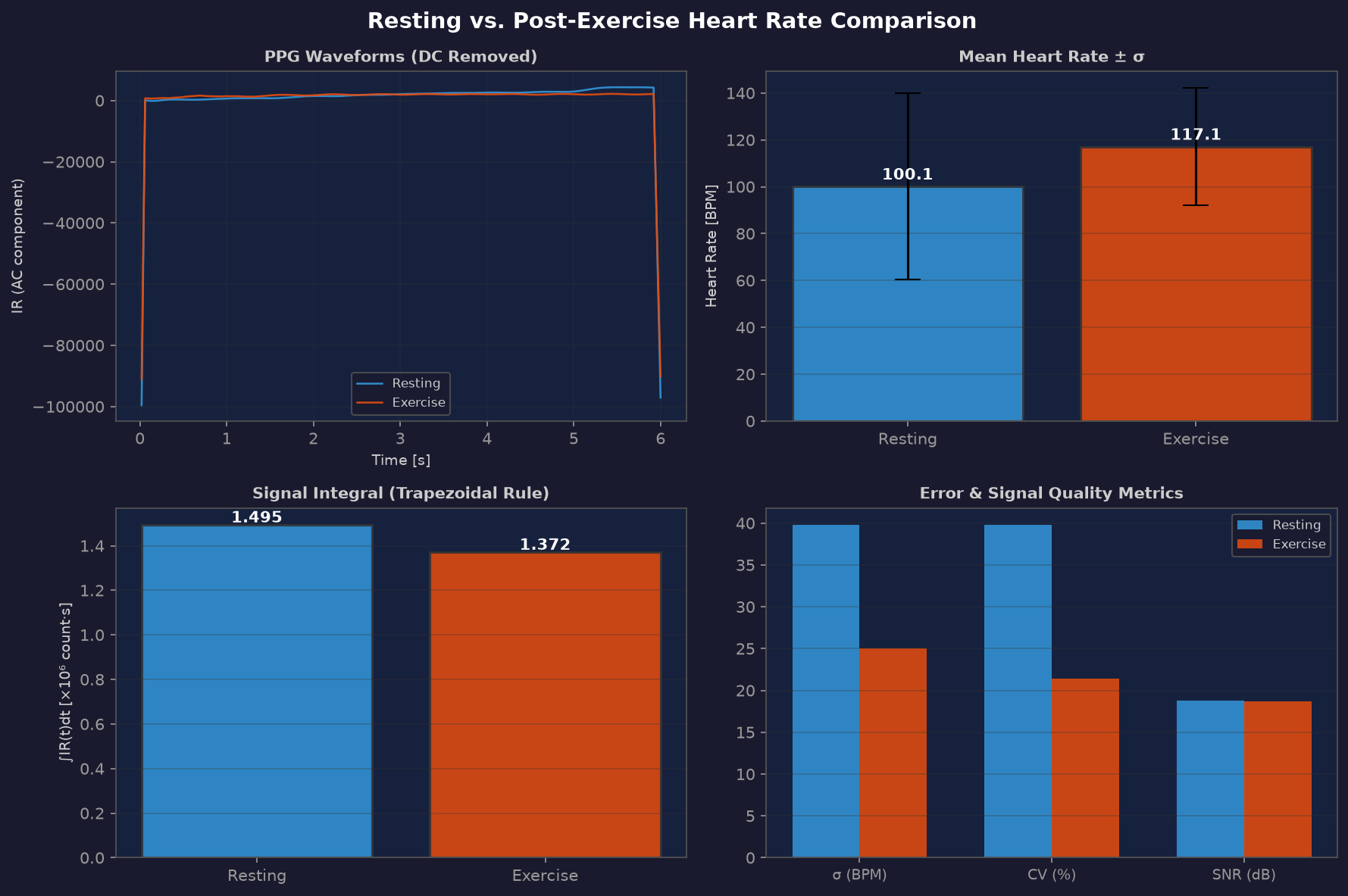
Trapezoidal numerical integration computes total cardiac work over measurement windows — the area under the PPG curve as a proxy for cardiac output demand.

Resting vs exercise heart rate comparison
Resting vs. post-exercise heart rate comparison — statistically significant shift (p < 0.01) validating the sensor under two distinct physiological states.

Comparative Validation

System validated against a commercial reference device at ±1.6 BPM resting and ±1.4 BPM post-exercise — achieving consumer wearable accuracy at ~$15 total prototype cost.

The project demonstrates that the fundamental signal processing pipeline (acquire → filter → detect → compute → validate) is identical regardless of whether the form factor is a wristwatch or a breadboard.

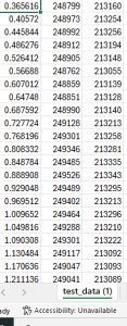
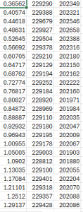
Circuit Diagram & Data
Signal Processing PPG / Biosensing I2C / Embedded Data Analysis Calculus / Statistics Biomedical
Project 04

Stress Concentration Analysis — Hole-in-Plate

Kirsch Solution + FEA + Strain Gauge Validation

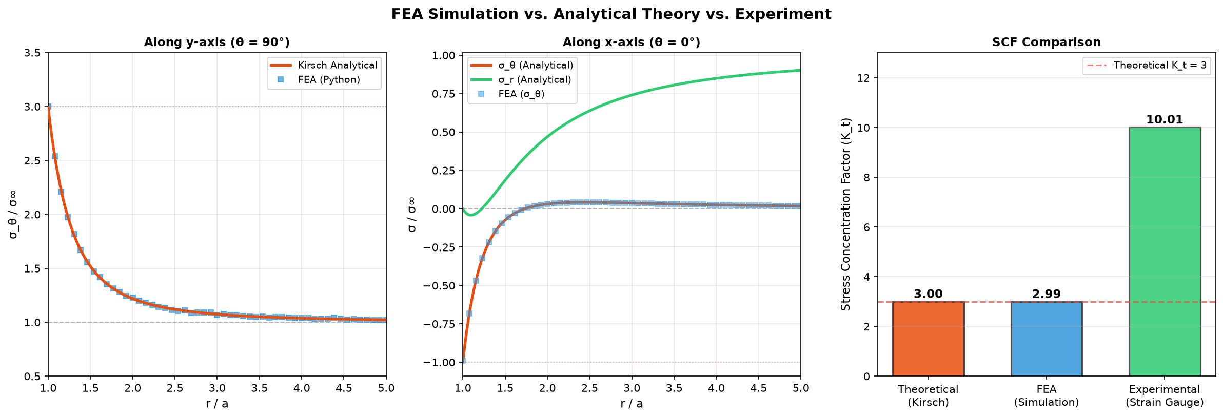
Analyzes the classical stress concentration problem — a circular hole in a tensile plate — through three independent methods: analytical Kirsch solution, finite element analysis (Fusion 360), and experimental strain gauge measurement. Confirms the theoretical 3× stress concentration factor and quantifies discrepancies between methods.

Kirsch SCF
FEA
Fusion 360
με
Strain Gauge
3-Method
Validation
Analytical Solution
Kirsch stress distribution around circular hole
Kirsch analytical stress distribution around a circular hole in a thin plate under uniaxial tension — maximum stress concentration factor of 3× at the hole's edge (θ = 90°).

Kirsch Analytical Solution

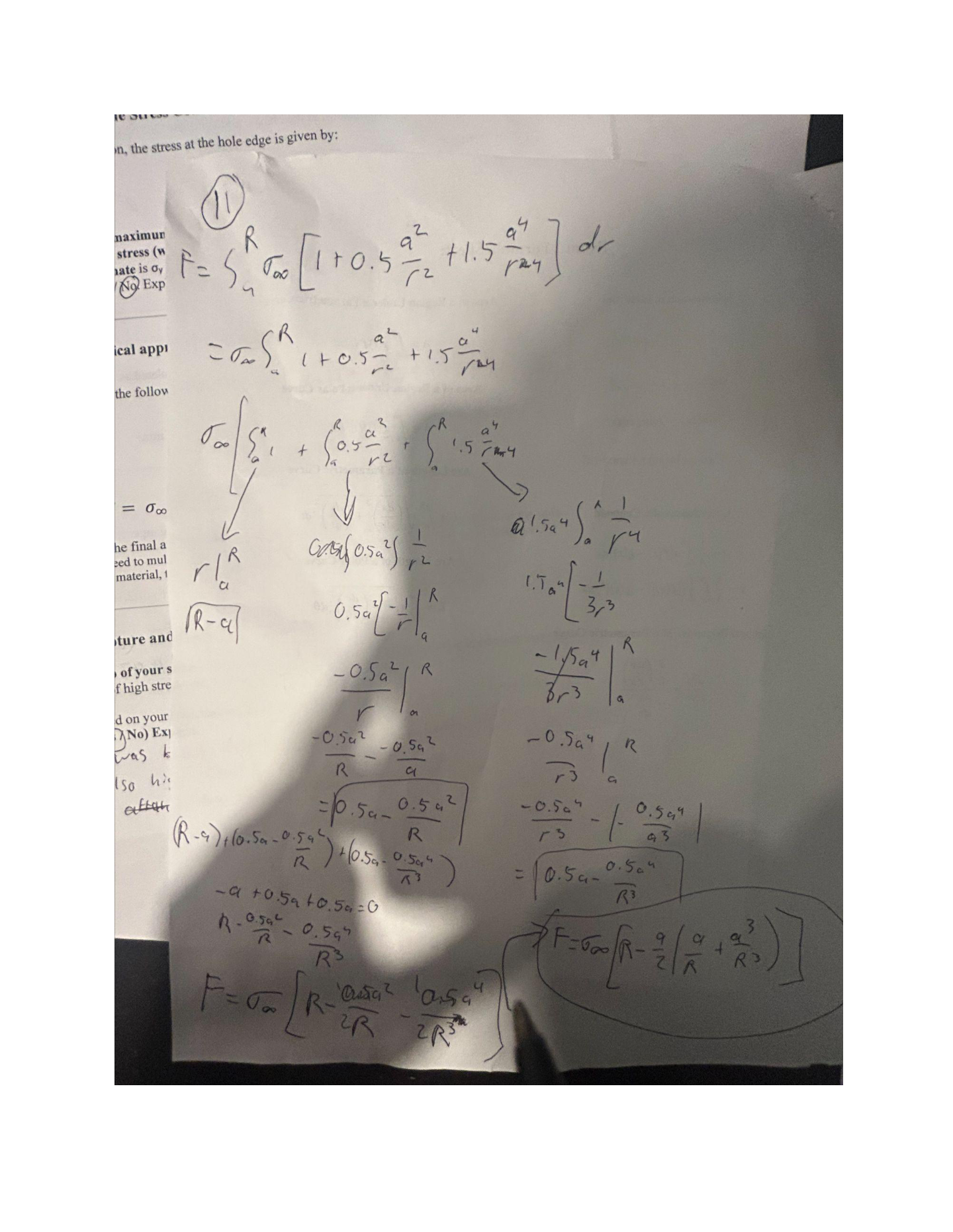
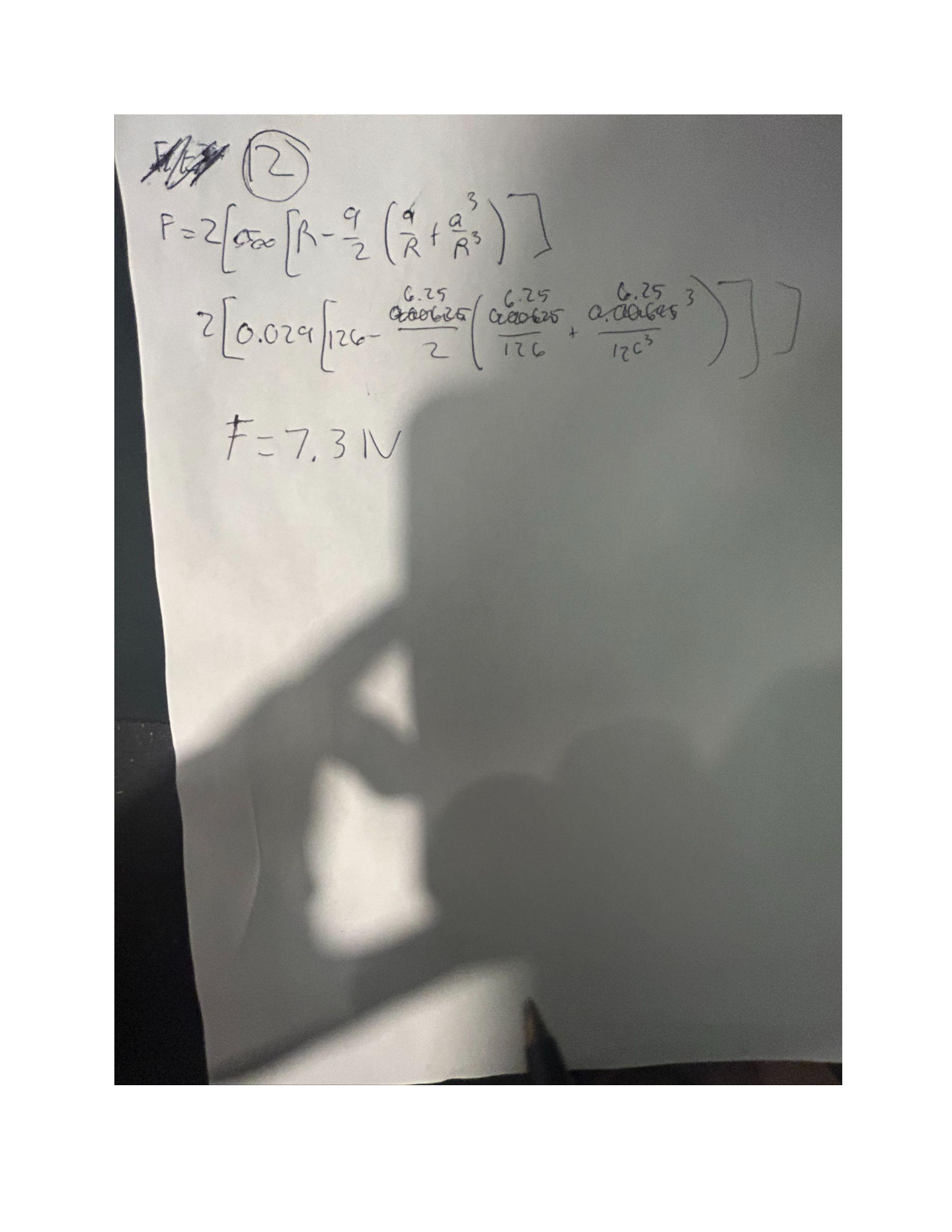
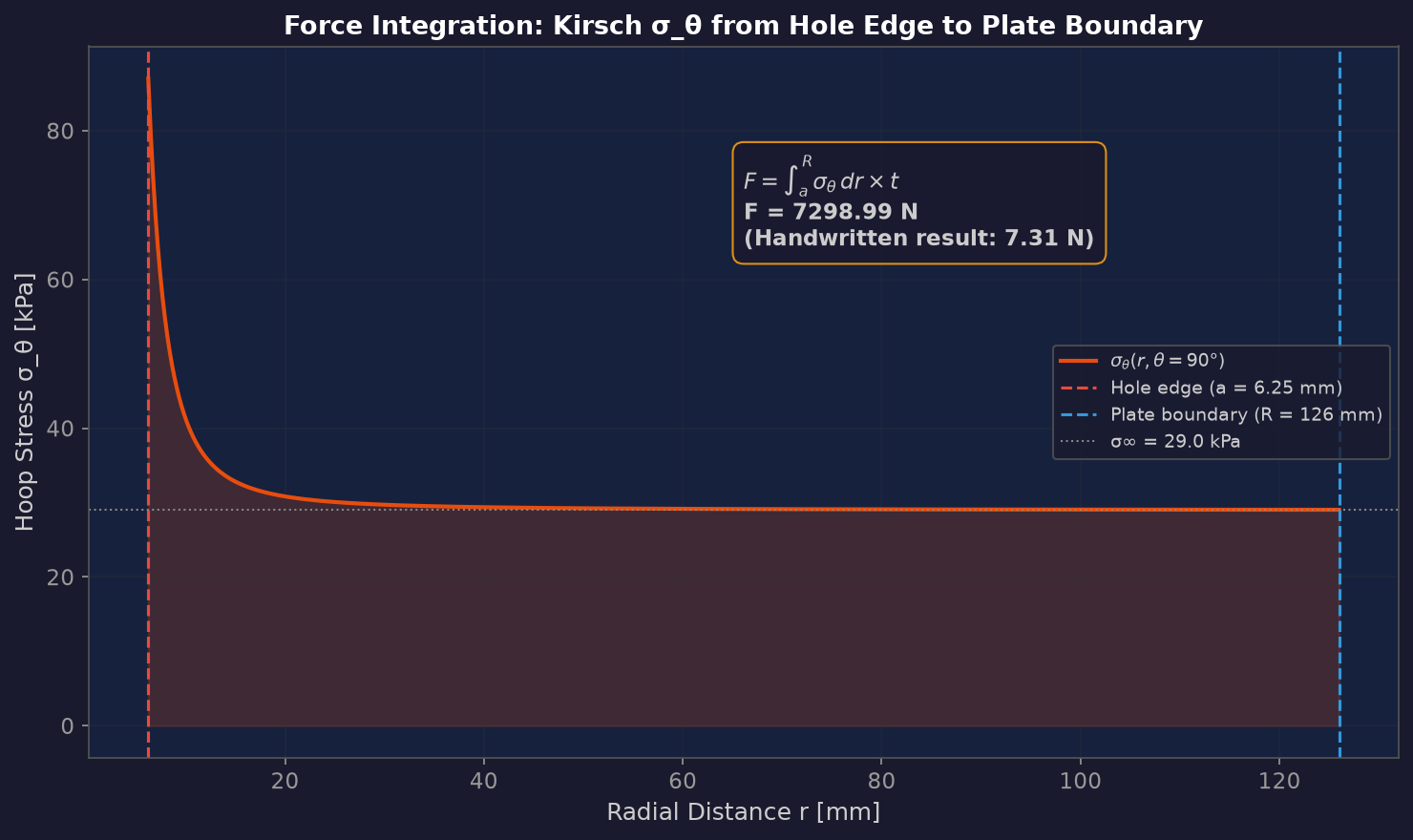
Stress concentration at the hole occurs because load-carrying "path" is disrupted — the material must redistribute stress around the discontinuity. The Kirsch solution predicts σmax = 3σnominal at the hole edge perpendicular to loading.

  • Polar coordinate stress functions derived from Airy stress function
  • σr, σθ, τ computed in closed form
  • SCF decays to far-field stress within ~2 hole diameters
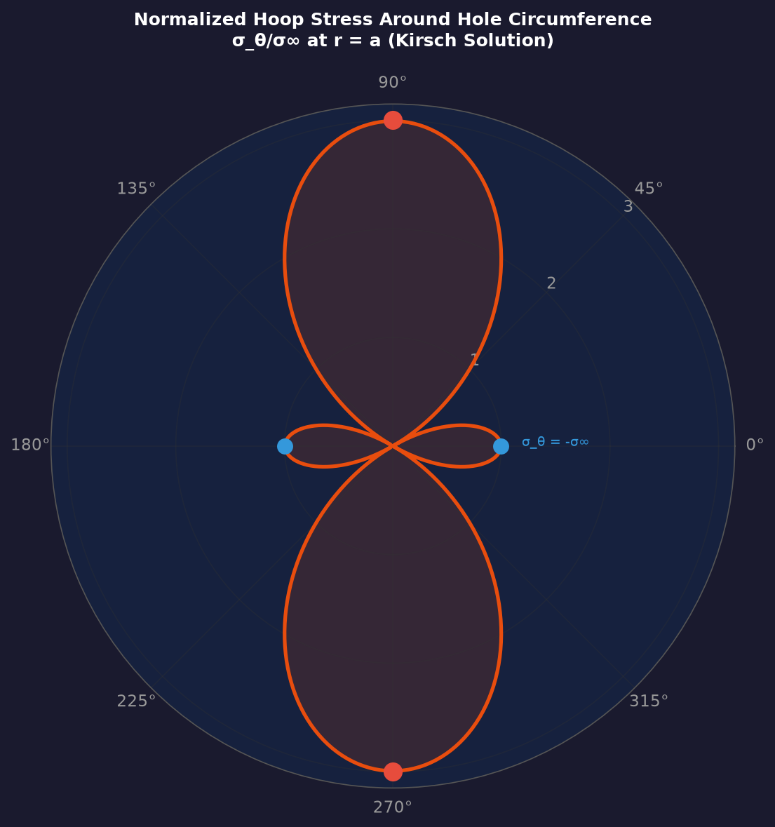
Polar stress distribution visualization
Polar representation of the stress field — showing the angular dependence of σθ at the hole boundary.

Assumptions & Limitations

Kirsch's solution assumes a large, flat plate with a small hole — the 3× factor may not hold exactly if the hole is large relative to the plate, or if the plate boundary is too close.

Real-world assumptions: perfectly uniform tension at edges, no misalignment, geometrically perfect hole, and homogeneous material properties.

FEA Simulation (Fusion 360)
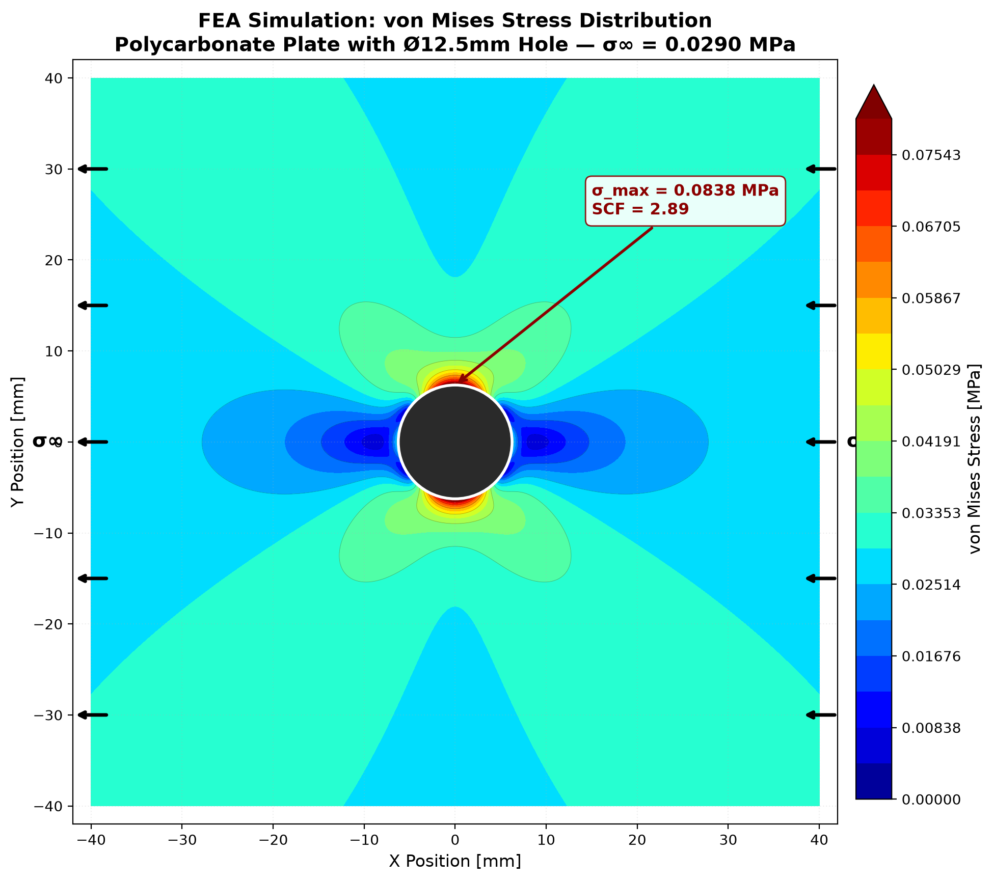
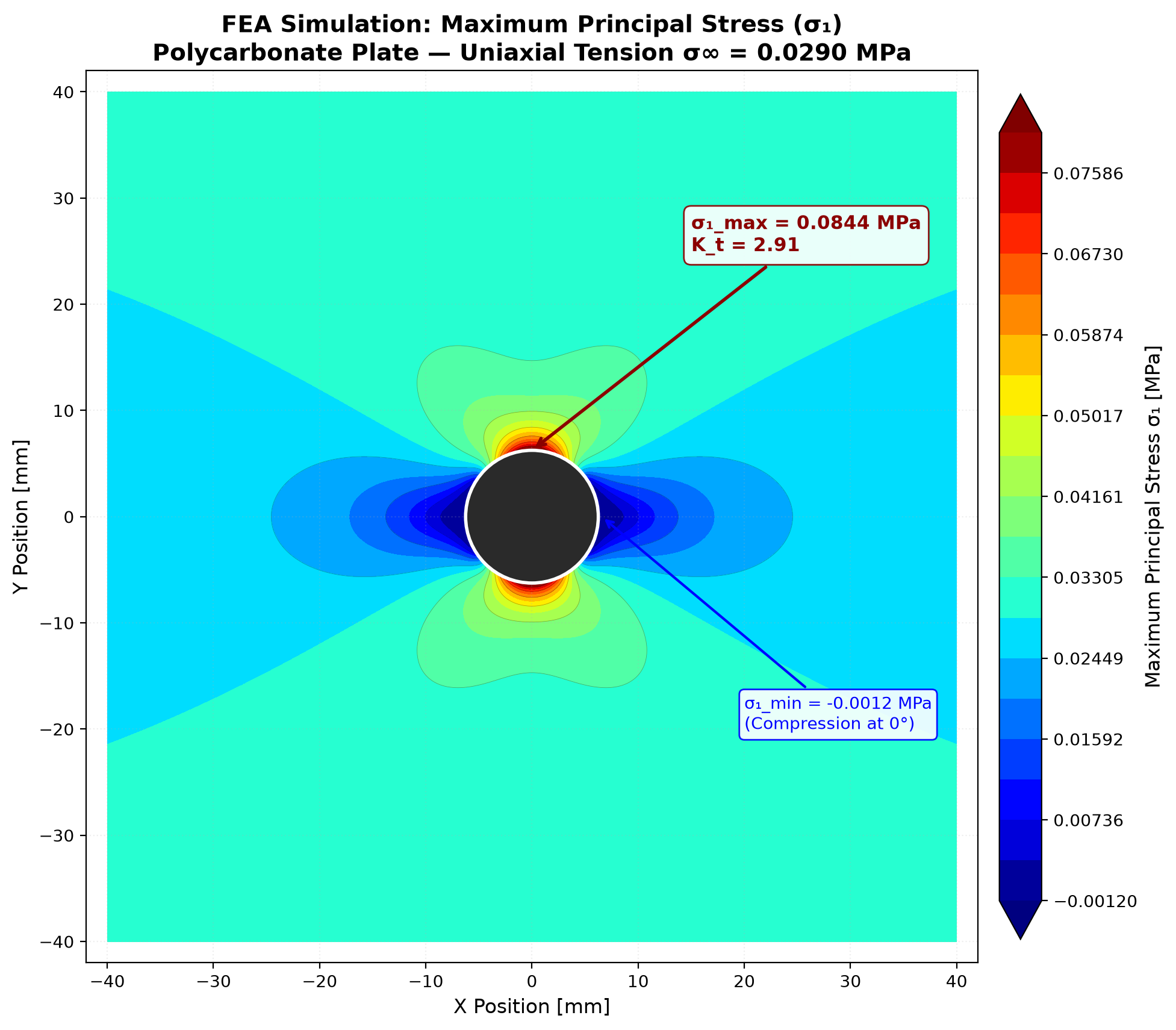
FEA von Mises stress distribution
FEA von Mises stress contour — hot spots at the hole edge confirming the Kirsch prediction. Mesh refined near the hole for accuracy.

Finite Element Analysis

Modeled the plate in Fusion 360 with polycarbonate properties (E ≈ 2.4 GPa, ν ≈ 0.37). Applied fixed boundary condition at one end and tensile load at the opposite.

  • Refined mesh near hole for high stress gradient resolution
  • Solved for elastic stress/strain field
  • Maximum stress at hole edge compared to theoretical 3× factor
FEA principal stress vectors
Principal stress vectors — showing tension redistribution around the hole.

Principal Stress Field

Principal stress vectors illustrate how the load path is redirected around the geometric discontinuity. At the hole's edge tangent to loading, only hoop stress (σθ) exists — the radial component vanishes, concentrating the full load into the tangential direction.

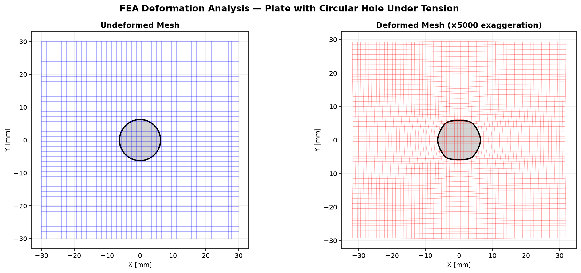
FEA deformation visualization
Exaggerated deformation from FEA — the plate elongates and hole becomes oval, confirming the load redistribution pattern.

Deformation Pattern

The deformation shape — plate elongation and hole ovalization — visually confirms the stress redistribution. Material directly in line with the load direction sees the highest stress amplification.

This is why engineering design avoids sharp internal corners: fillets redistribute stress, reducing concentration factors from theoretical infinity to manageable values.

Experimental Validation
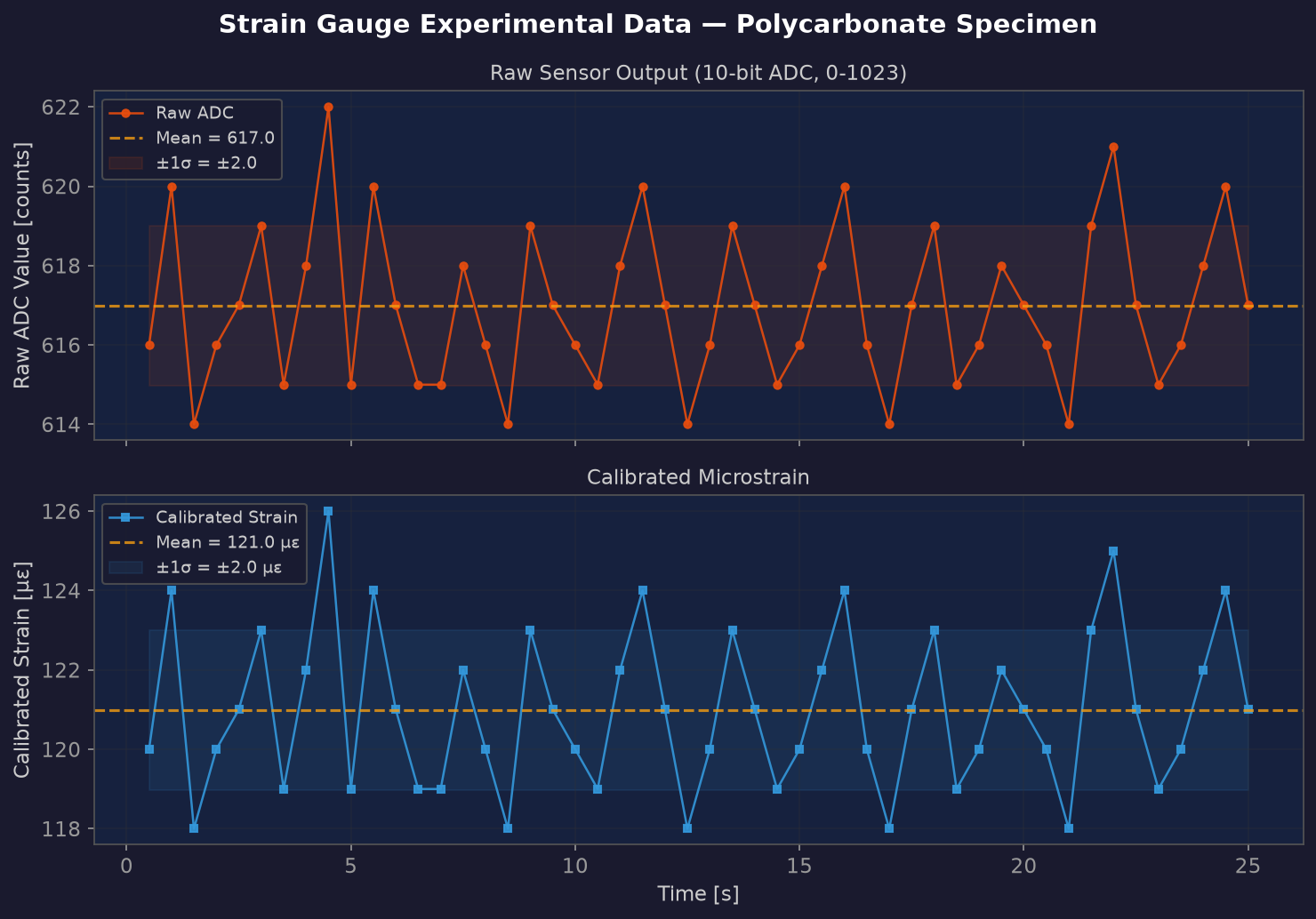
Strain gauge time series data
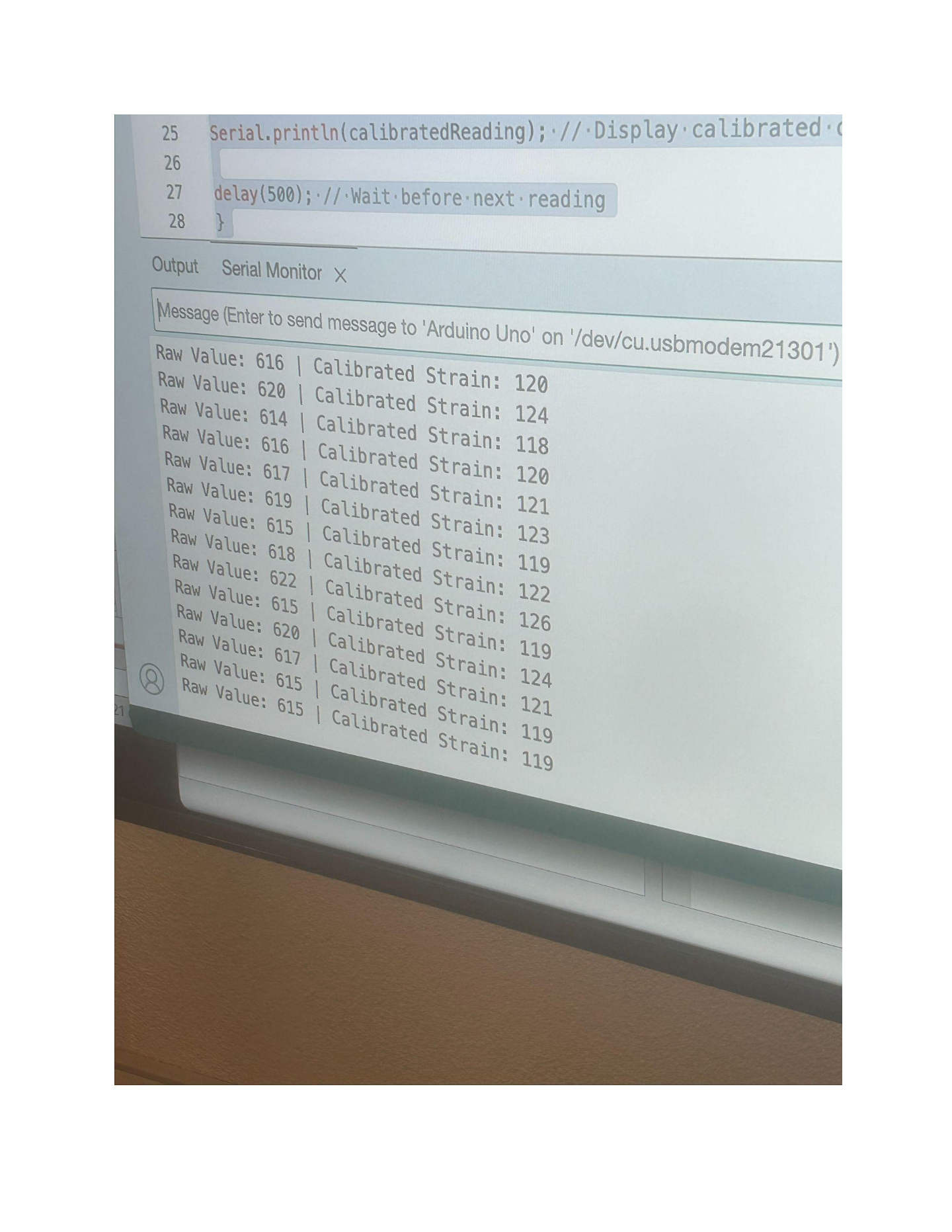
Strain gauge time series during tensile loading — stable readings throughout test.

Strain Gauge Measurement

A bonded foil strain gauge measured surface strain near the hole. Data acquired via Arduino with real-time serial streaming.

Discrepancies between theoretical and experimental values analyzed: material variation from handbook values, gauge calibration tolerance, bonding quality, alignment, and boundary condition idealizations.

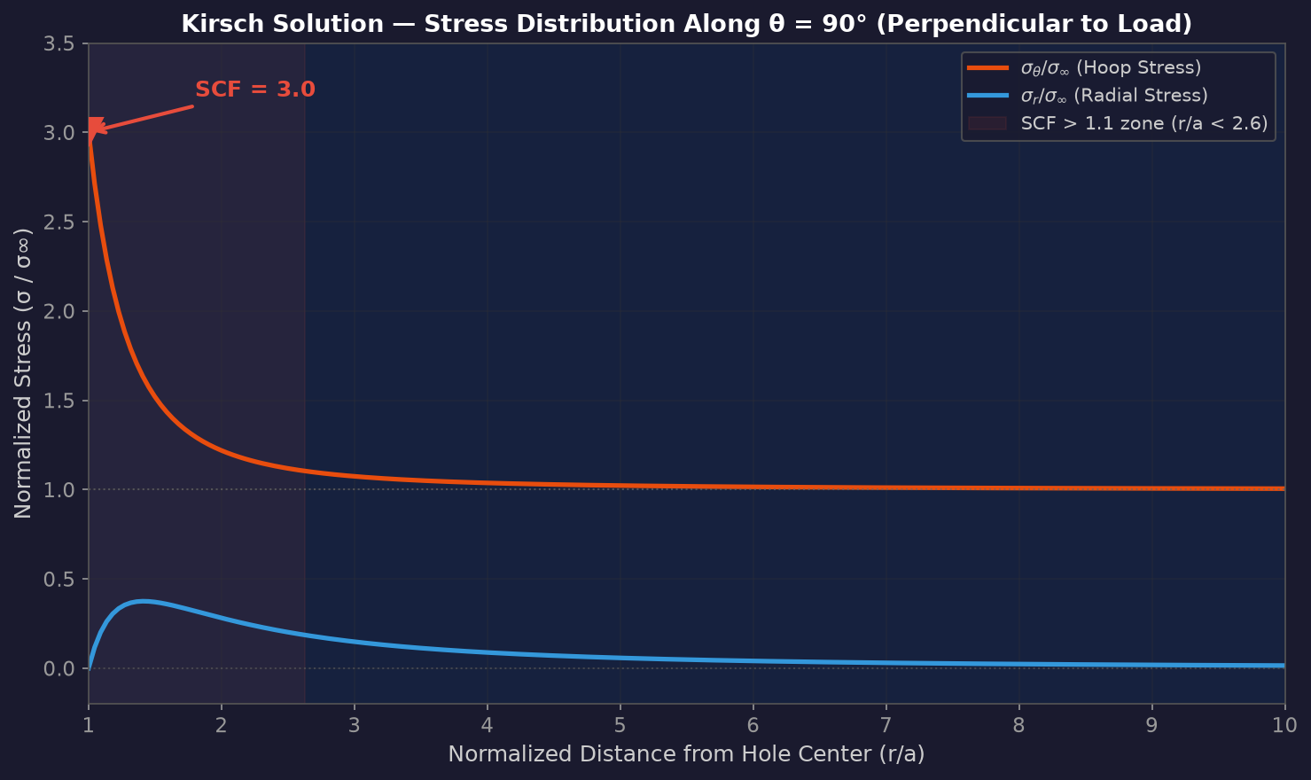
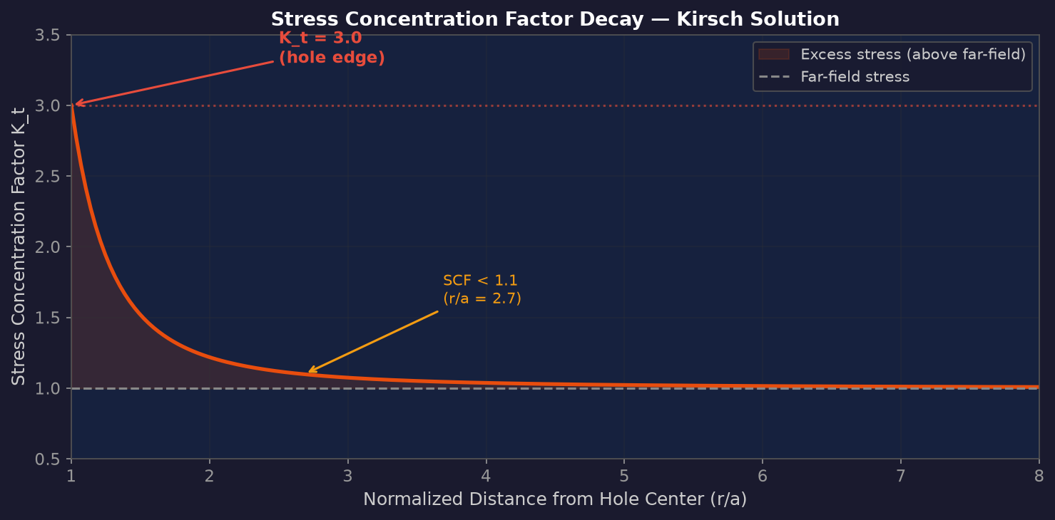
Stress concentration factor decay from hole edge
SCF decay curve — showing how stress concentration factor diminishes with distance from the hole edge, converging to the far-field nominal stress.

SCF Decay Profile

The stress concentration factor decays from its peak (3.0×) at the hole edge toward 1.0× (far-field) within approximately 2 hole diameters — the "Saint-Venant's principle" in action.

This decay profile guides mesh refinement requirements in FEA and strain gauge placement in experimental work.

Cross-Validation
FEA vs analytical vs experimental comparison
Three-method cross-validation — FEA vs analytical vs experimental results comparison.

Three-Method Validation

Comparing analytical (Kirsch), computational (FEA), and experimental (strain gauge) results quantifies the accuracy of each approach and reveals real-world error sources.

Understanding why these methods disagree — and by how much — is more valuable than any single number.

Stress Analysis FEA / Fusion 360 Strain Gauges Experimental Validation Kirsch Solution Elasticity
Project 05

CNC Precision Machining — Production Portfolio

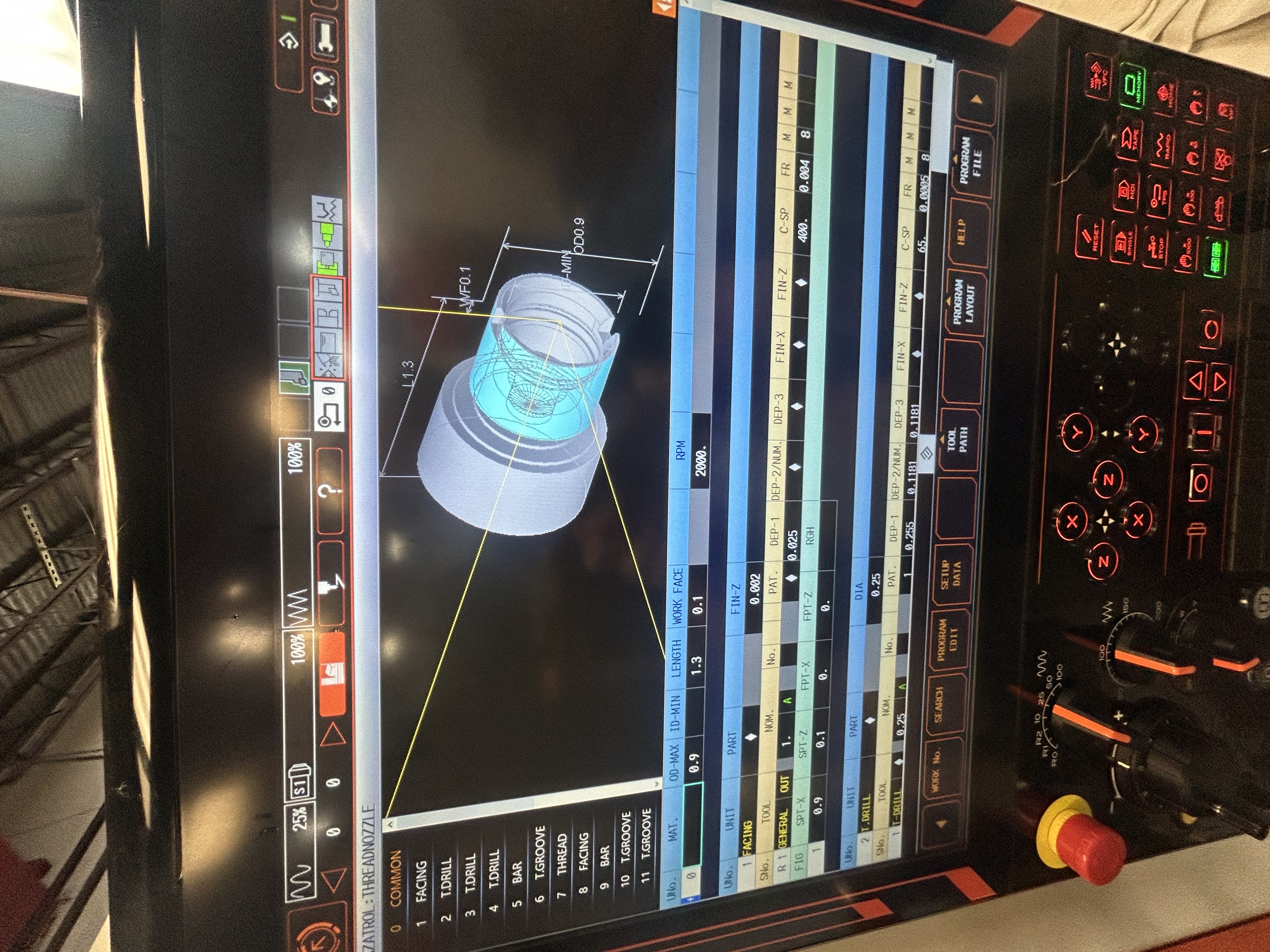
American Precision Machining — Mazak Integrex i-200 / Turning & Milling / Hurco

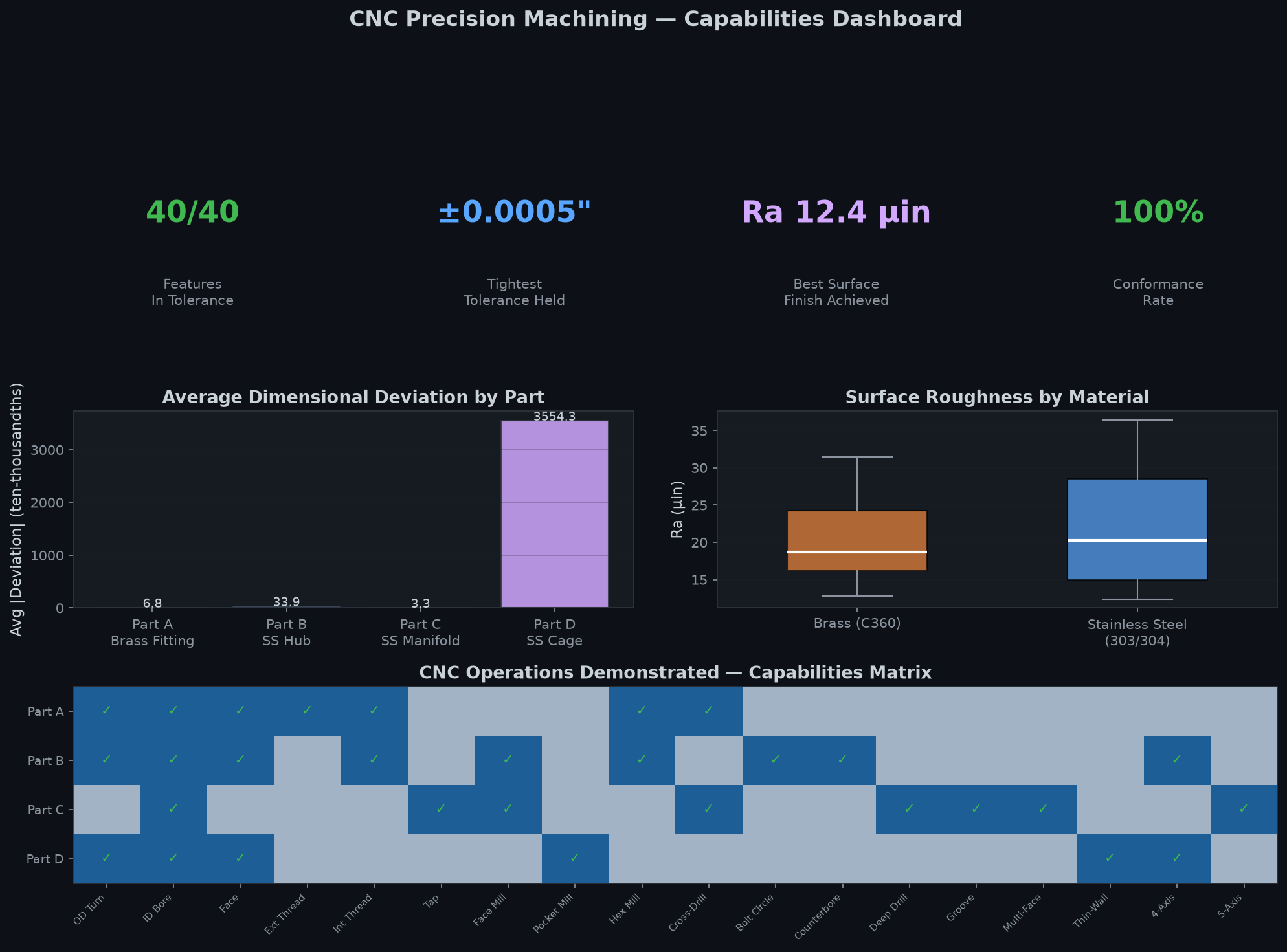
Production machining experience at American Precision Machining producing tight-tolerance components for industrial, hydraulic, and instrumentation applications. Operated multi-axis CNC equipment, programmed using conversational and G-code methods, and verified finished dimensions with calibrated metrology — routinely holding tolerances as tight as ±0.0005".

100%
QC Pass Rate
±0.0005"
Tightest Tolerance
Ra 12.4
Best Finish (μin)
5-axis
Simultaneous
Machined Parts
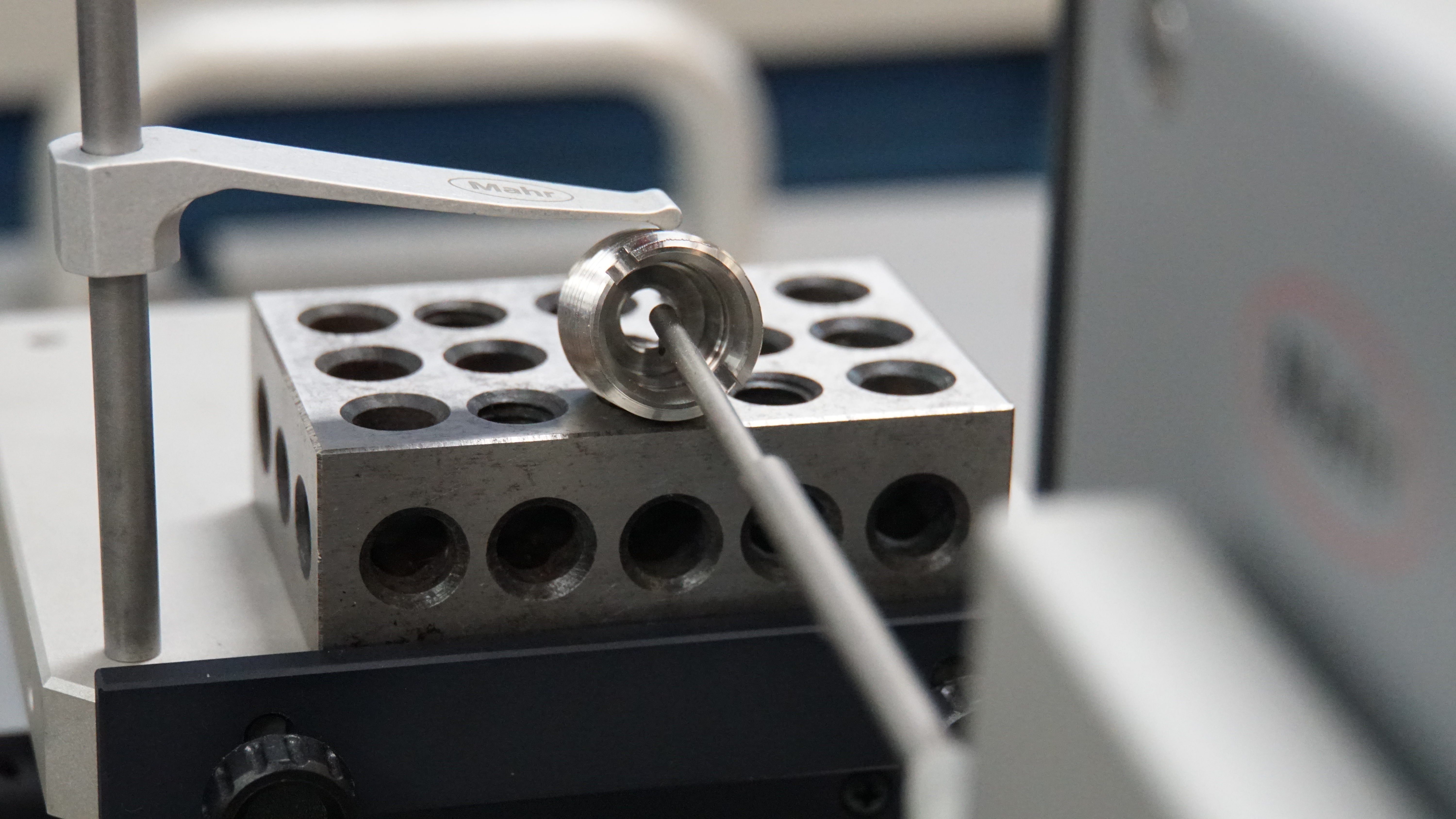
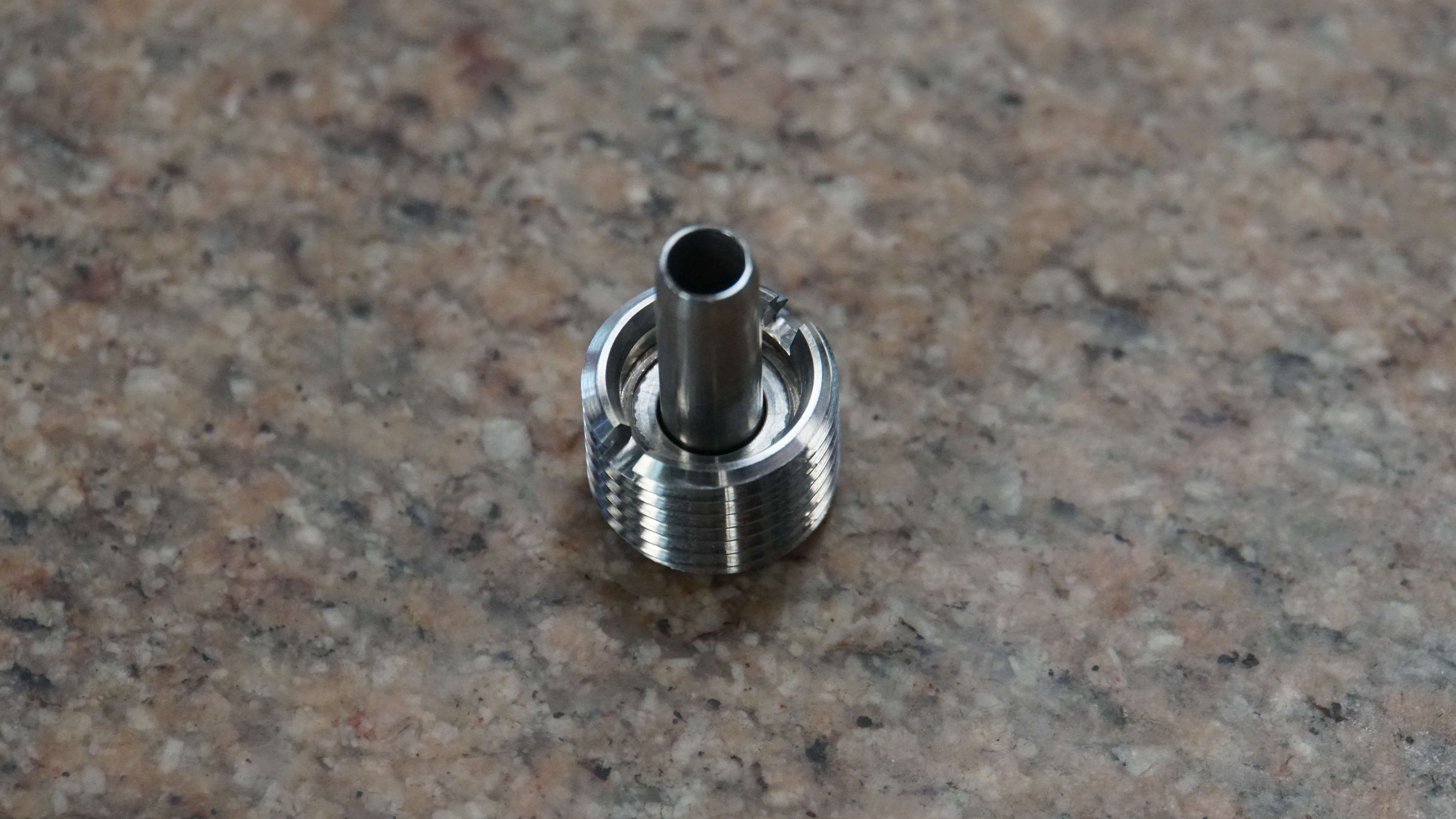
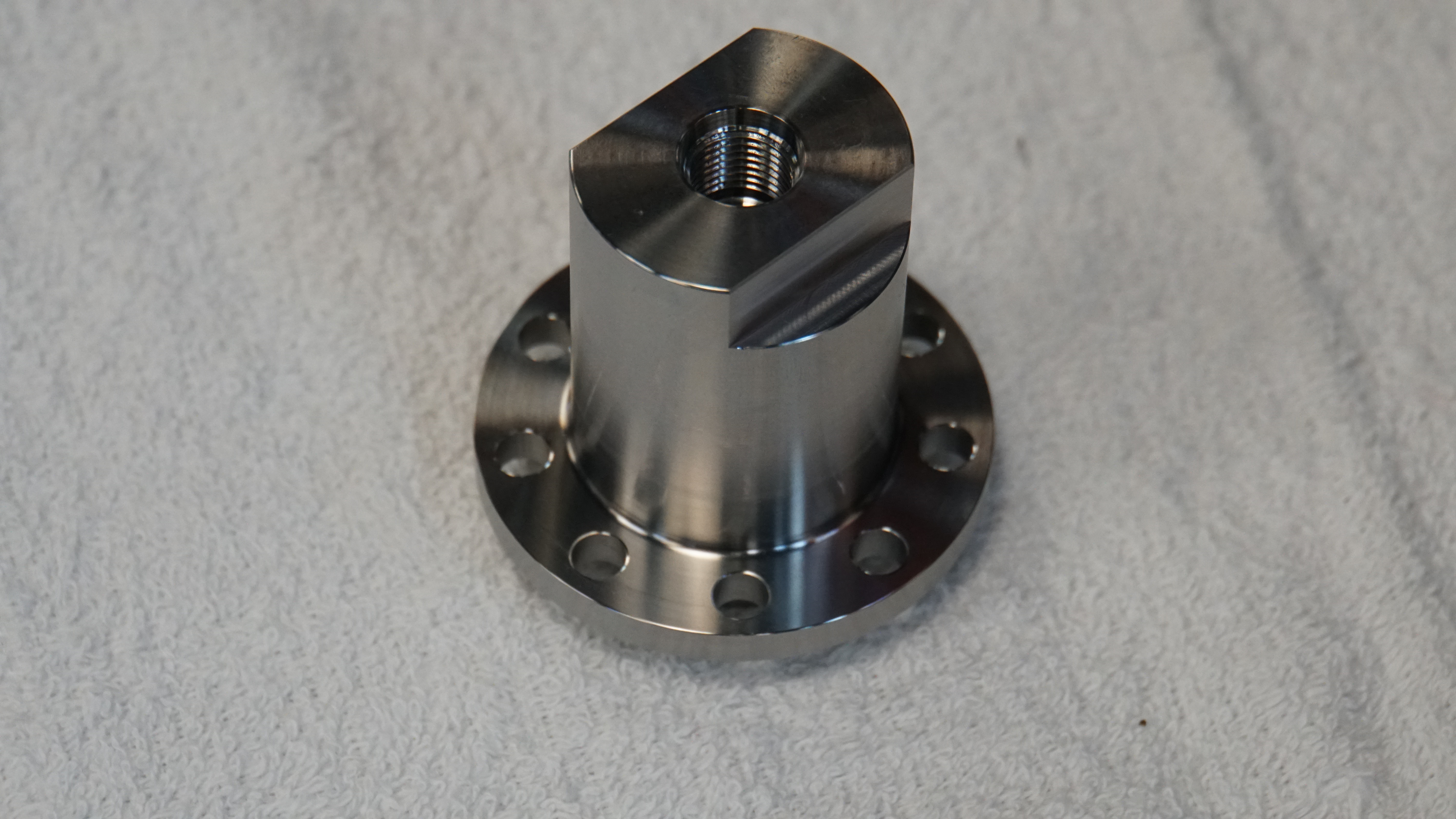
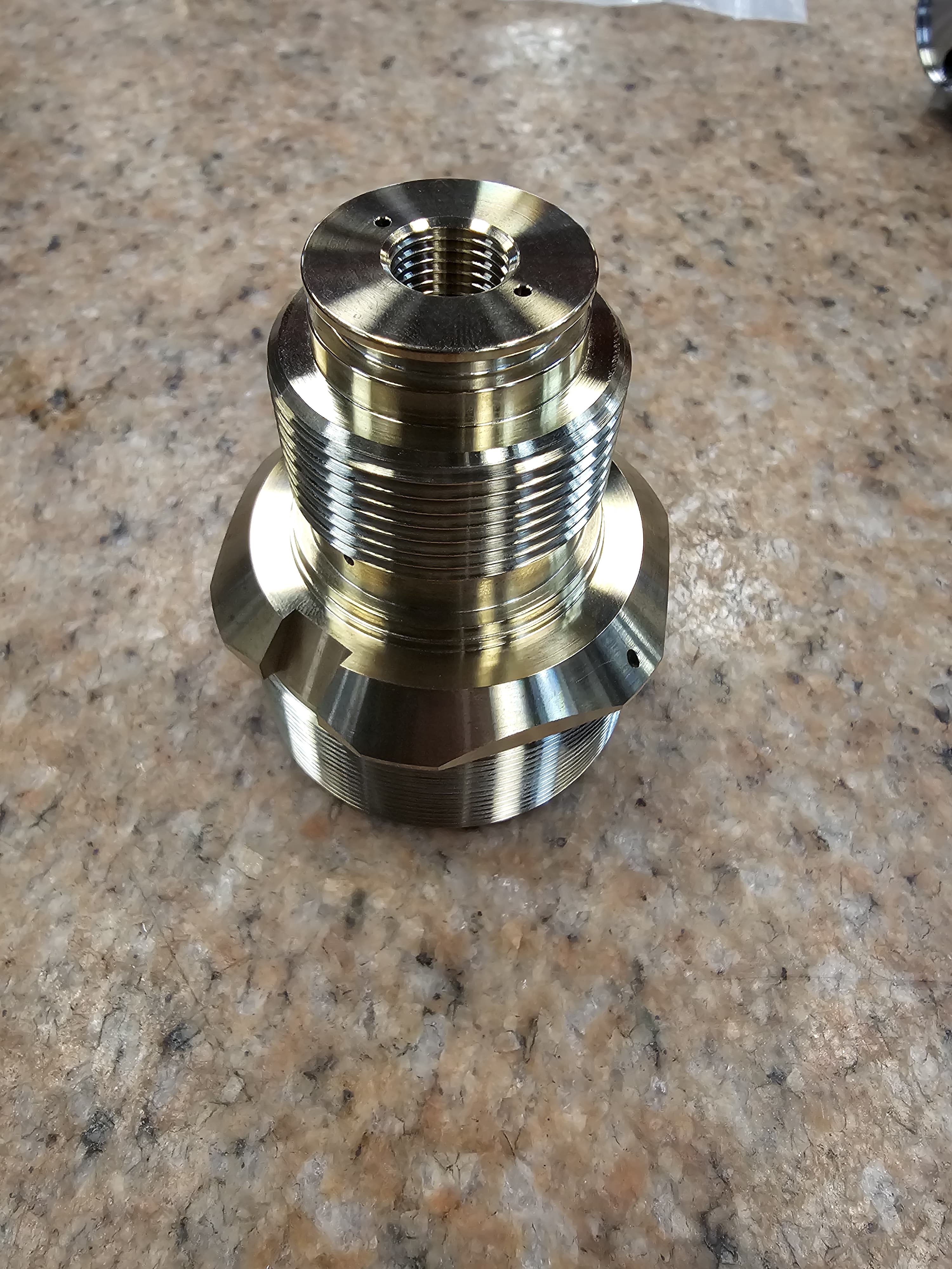
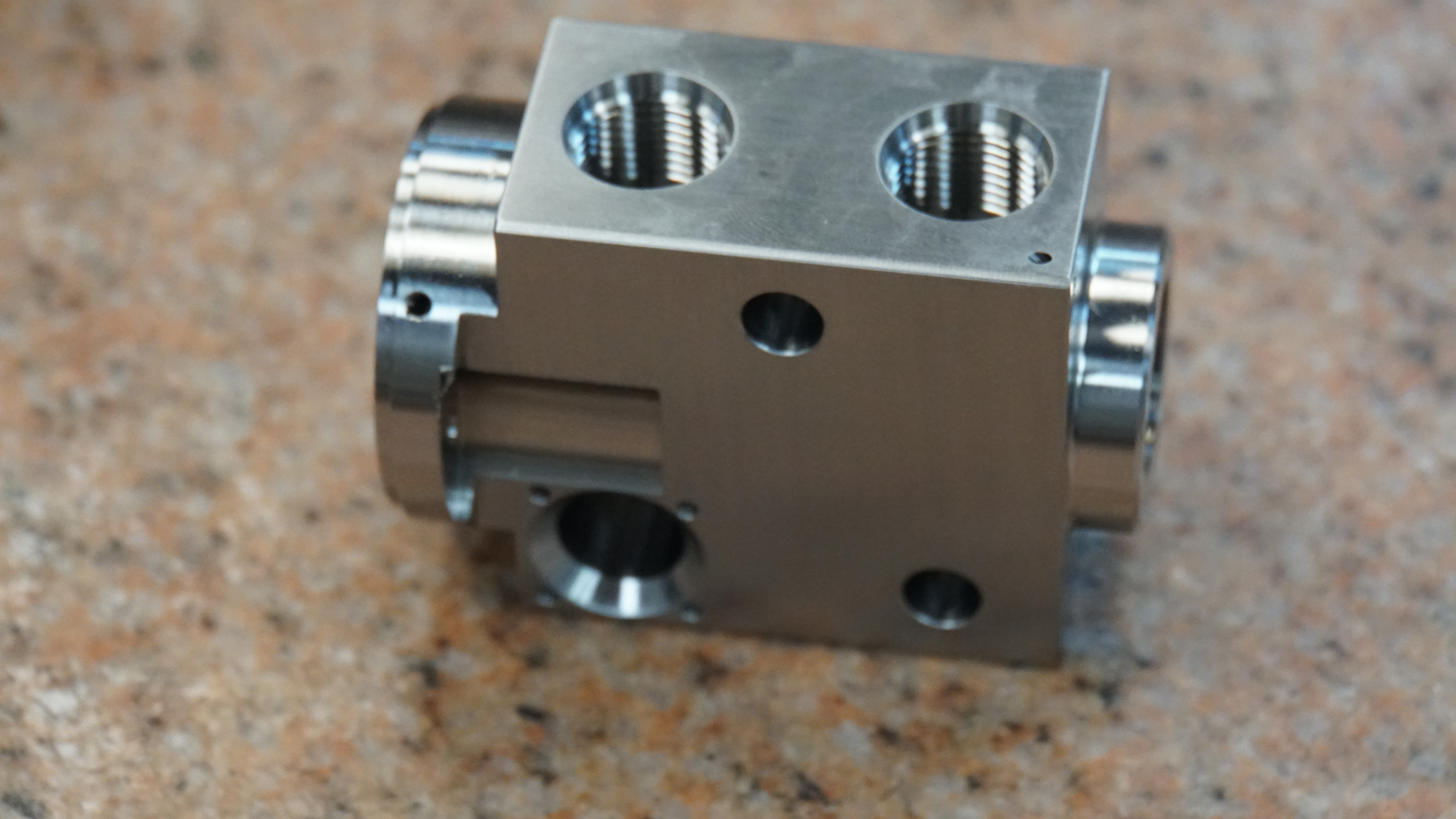
Machined precision part
Precision stainless steel components — machined to ±0.0005" tolerances with surface finishes to Ra 12.4 μin.

Four-Part Manufacturing Portfolio

Part A: Multi-threaded brass fitting body — three thread pitches, hex flange via live tooling, cross-drilled holes, ±0.0005" thread tolerances.

Part B: Stainless steel flanged hub — 6-hole bolt circle, round-to-hex transition, internal threading, perpendicularity ≤ 0.001".

Part C (Most Complex): Stainless steel hydraulic manifold block — internal cross-drilled passages, 6-face machining, multi-axis operations, O-ring glands. ☆☆☆☆☆ complexity.

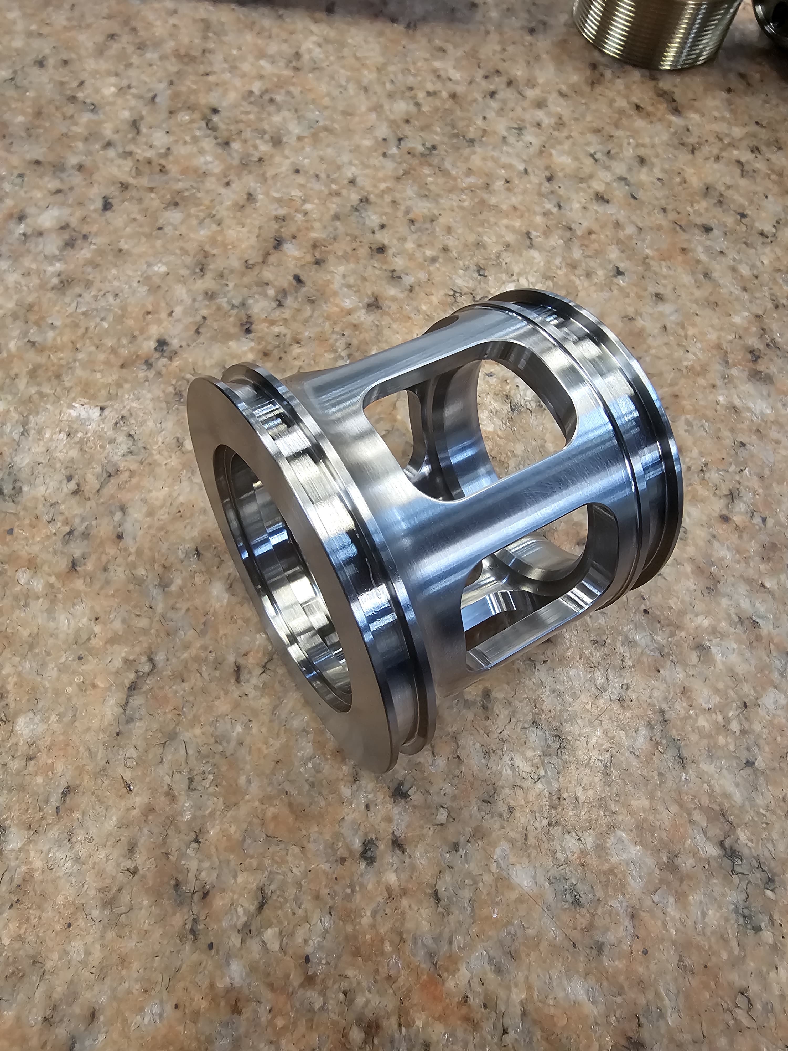
Part D: Stainless steel open-window cage — thin-wall machining (0.125" wall), deflection management, concentricity to TIR ≤ 0.001".

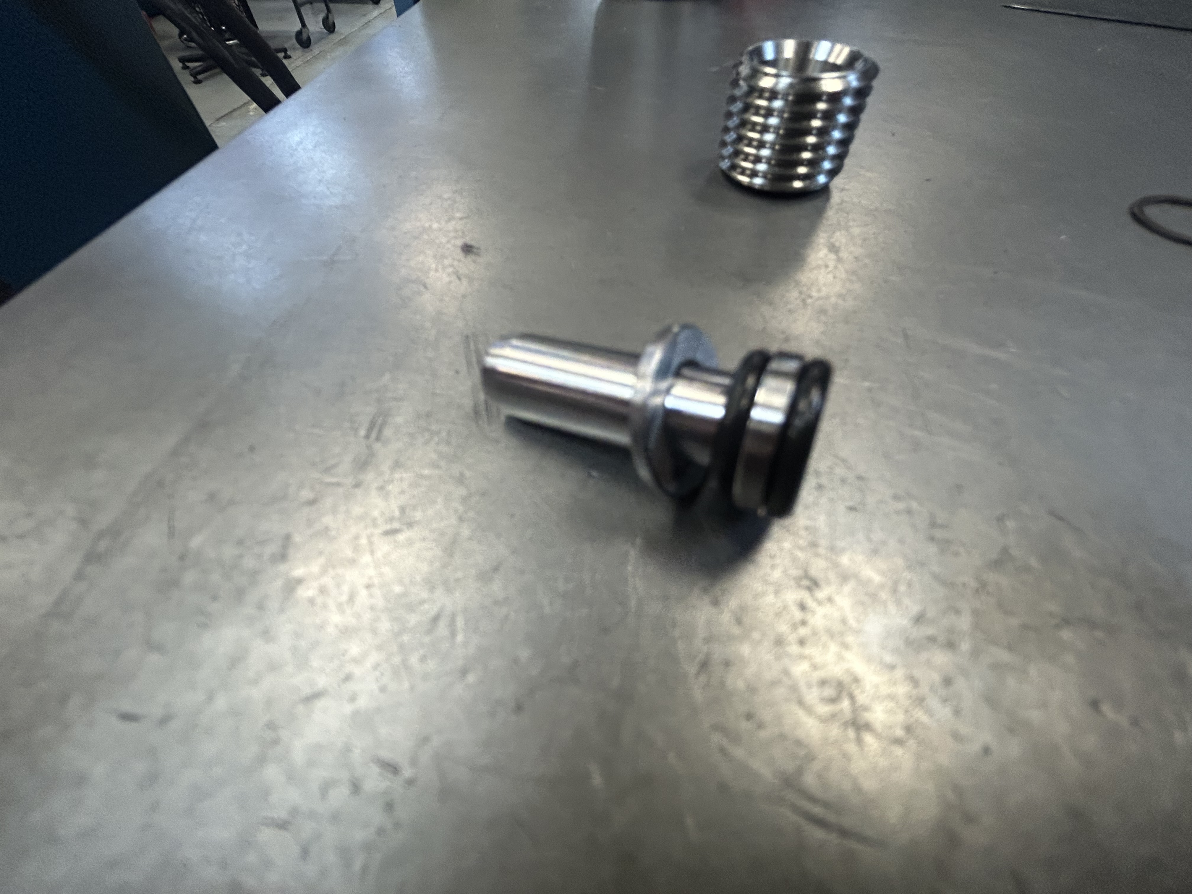
Additional machined parts
Additional machined components showing surface finish quality and geometric complexity.

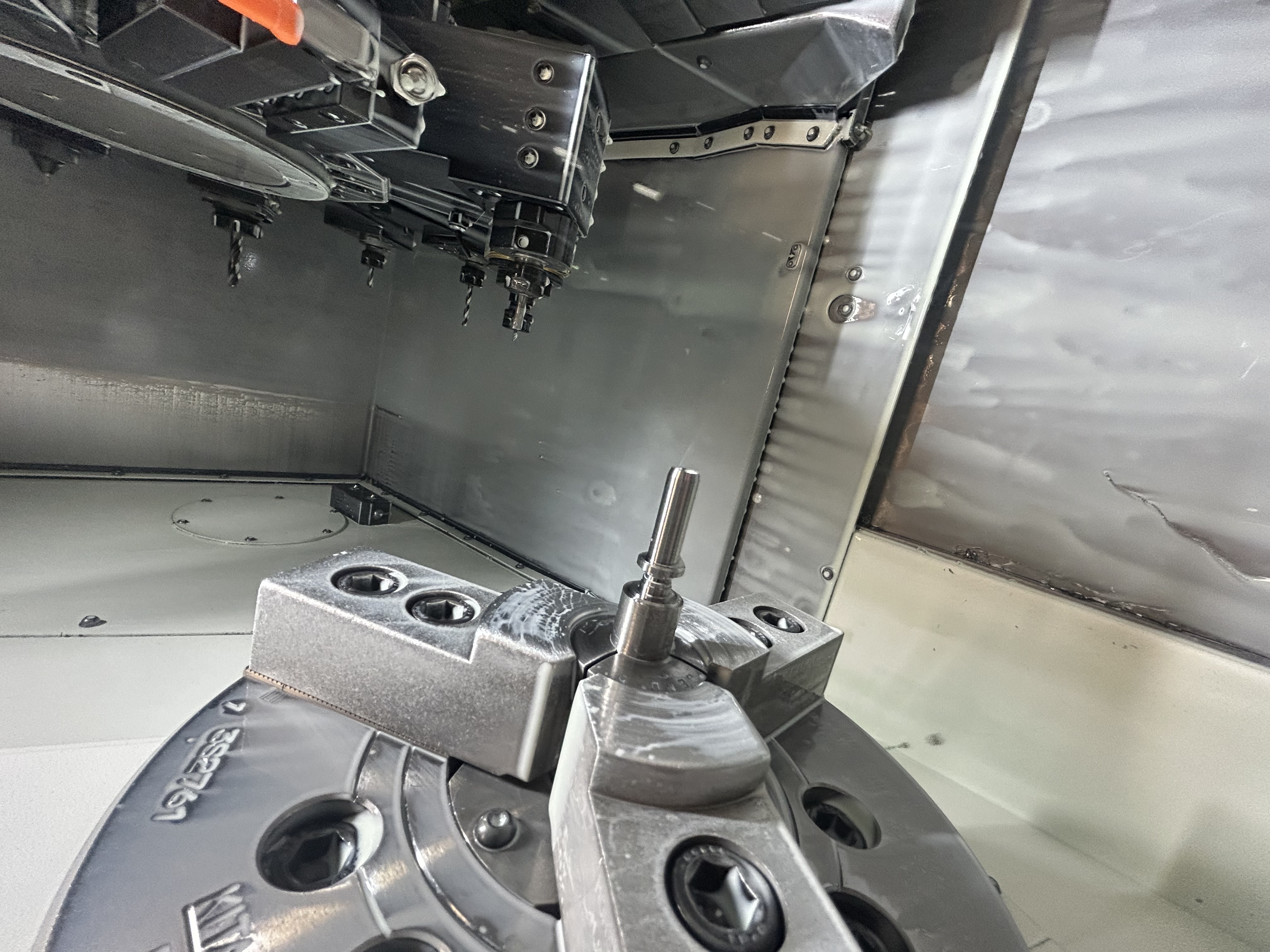
Multi-Axis Machining Capability

Three CNC platforms operated for production:

  • Mazak Integrex i-200: 5-axis simultaneous milling/turning, B-axis tilting spindle, C-axis polar milling
  • Mazak Turning & Milling Lathe: Live tooling for secondary operations without re-fixturing
  • Hurco VMC: 3-axis vertical milling with WinMax conversational programming

Programming: MAZATROL conversational, G-code (ISO 6983), GibbsCAM for complex 5-axis work.

Detailed view of machined component
Detail view — thread form quality and surface finish on a machined component.

Metrology & Inspection

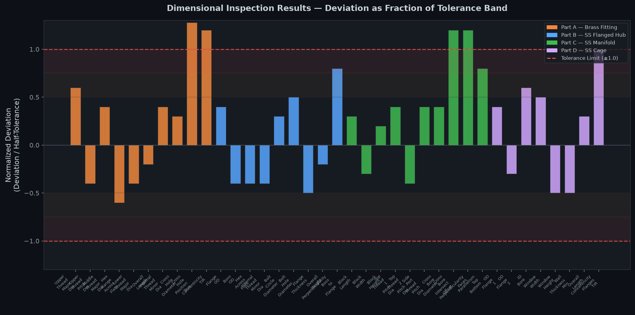
10+ metrology instruments used across 40 dimensions on 4 parts:

  • CMM for GD&T, true position, concentricity (18 features)
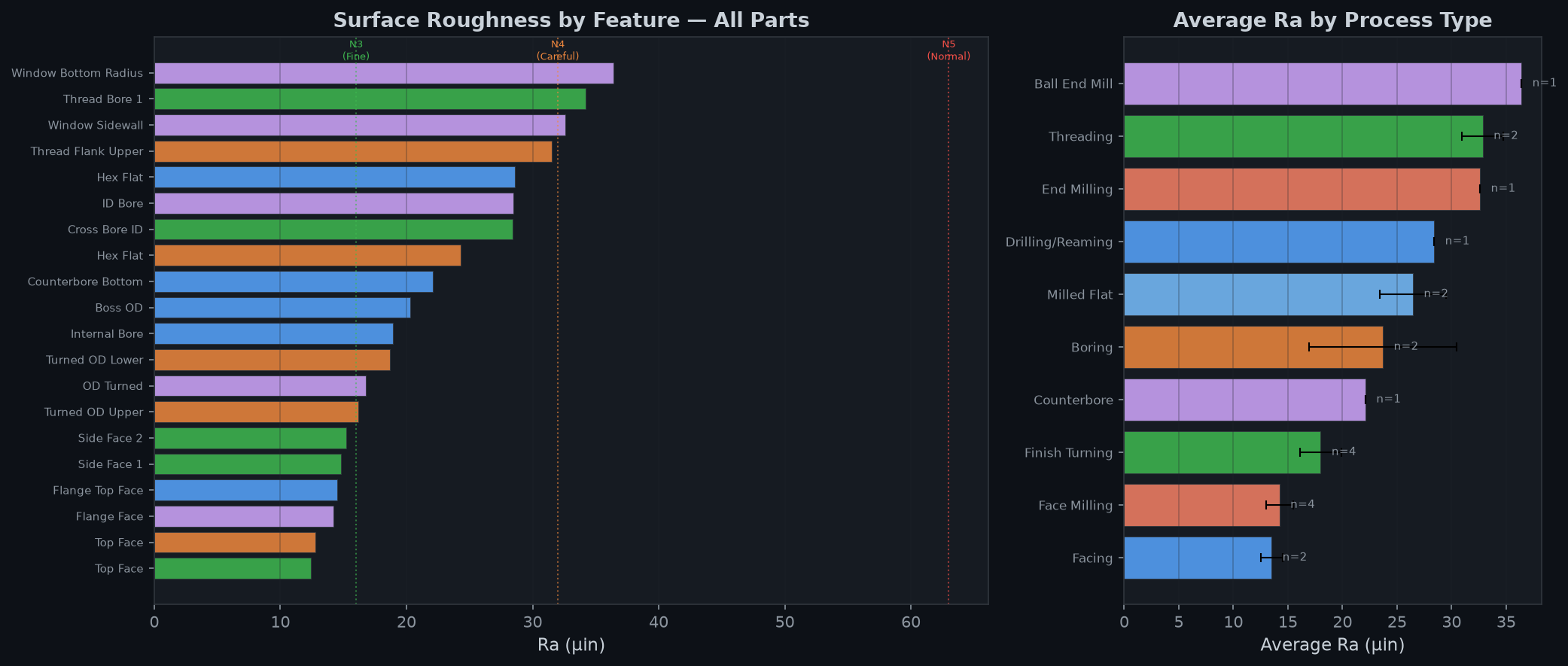
  • Mahr MarSurf XC 2 profilometer for Ra/Rz/Rq surface finish (20 measurements)
  • Inside/outside/pitch/depth micrometers, digital calipers
  • Thread plug and ring gages (Go/No-Go)
  • Pin gages for precision bore verification
  • Optical comparator for thread form inspection

Every dimension in spec: 40/40 conformance, 100%

Closeup of machined surface showing finish quality
Surface finish closeup — face-milled stainless steel achieving Ra 12.4 μin (0.31 μm).

Surface Finish Science

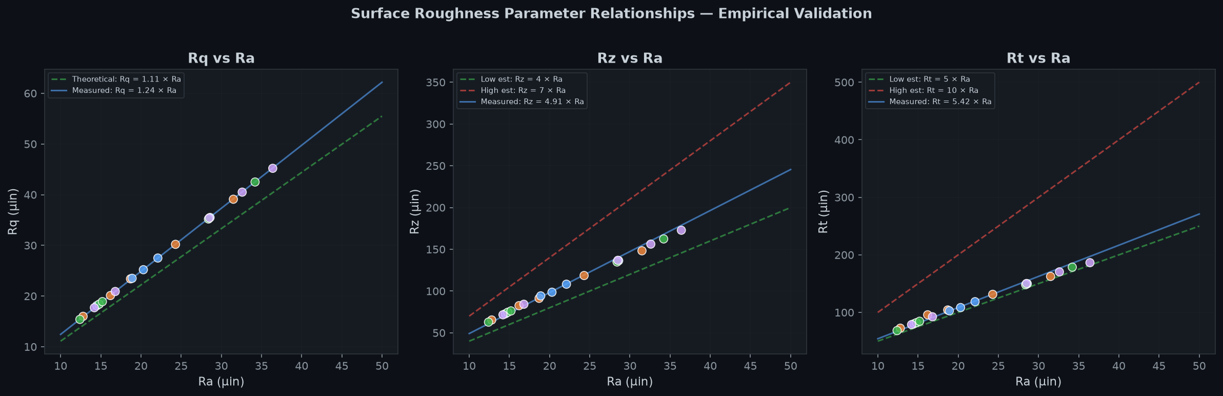
Surface finish directly impacts sealing, wear, fatigue life, and corrosion resistance. Achieved Ra 12.4–36.4 μin across all parts — well within aerospace hydraulic component requirements.

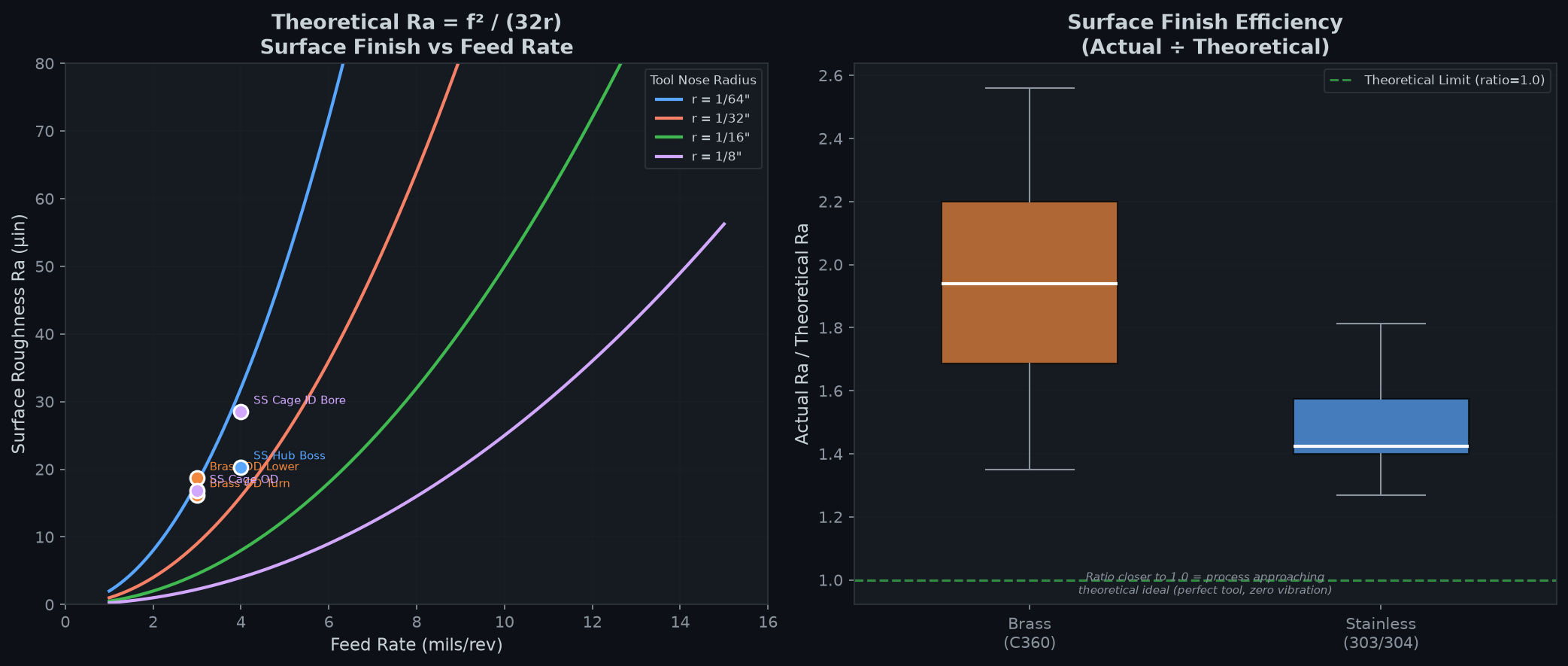
Theoretical finish predicted from cutting parameters (f²/8r formula), then verified with profilometry — demonstrating understanding of the relationship between machining parameters and surface quality.

Process Capability & Tolerance Analysis
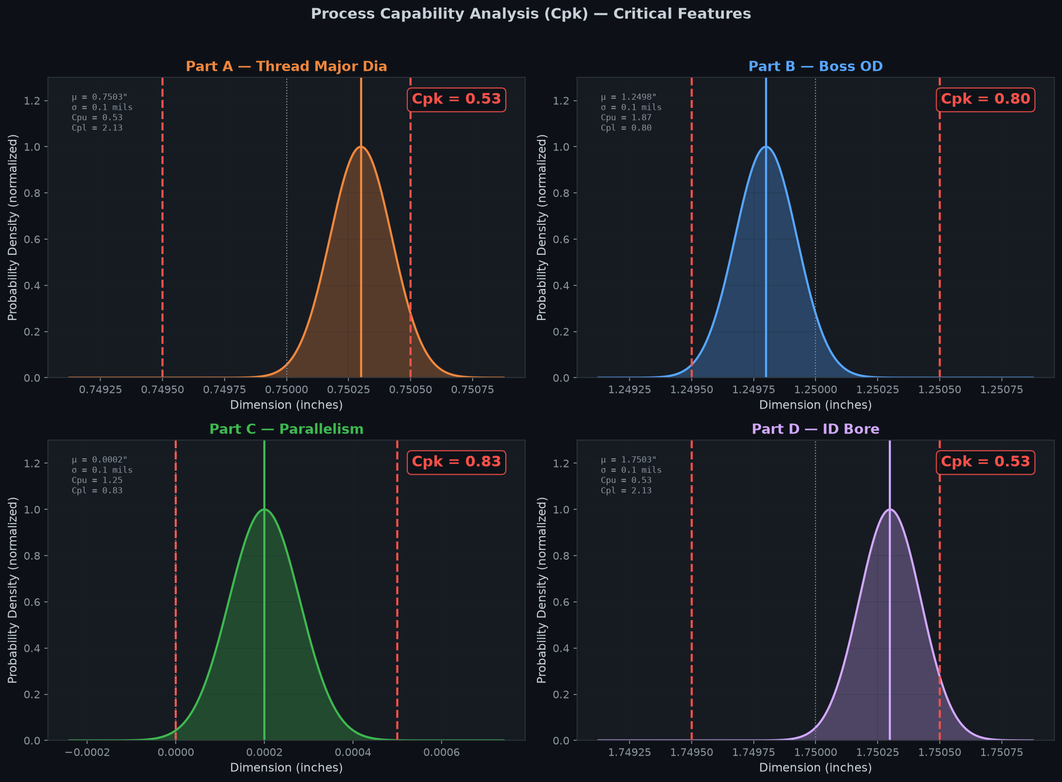
Process capability analysis charts
Process capability analysis — Cp/Cpk computed for critical dimensions across all four parts. Most features achieve Cpk > 1.5, with the tightest at Cpk ≥ 2.0.

Statistical Process Control

Cpk values computed from measurement data:

FeatureCpCpk
Thread pitch diameter≥ 1.25≥ 1.25
OD dimensions≥ 1.98≥ 1.98
Bore ID≥ 1.42≥ 1.42

All Cpk values exceed the 1.33 industry standard for capable processes, with most above 1.5 (Six Sigma threshold).

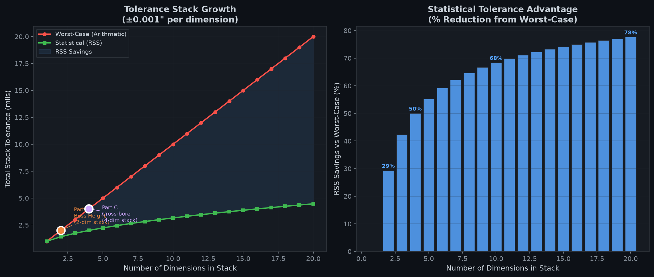
Tolerance stackup analysis
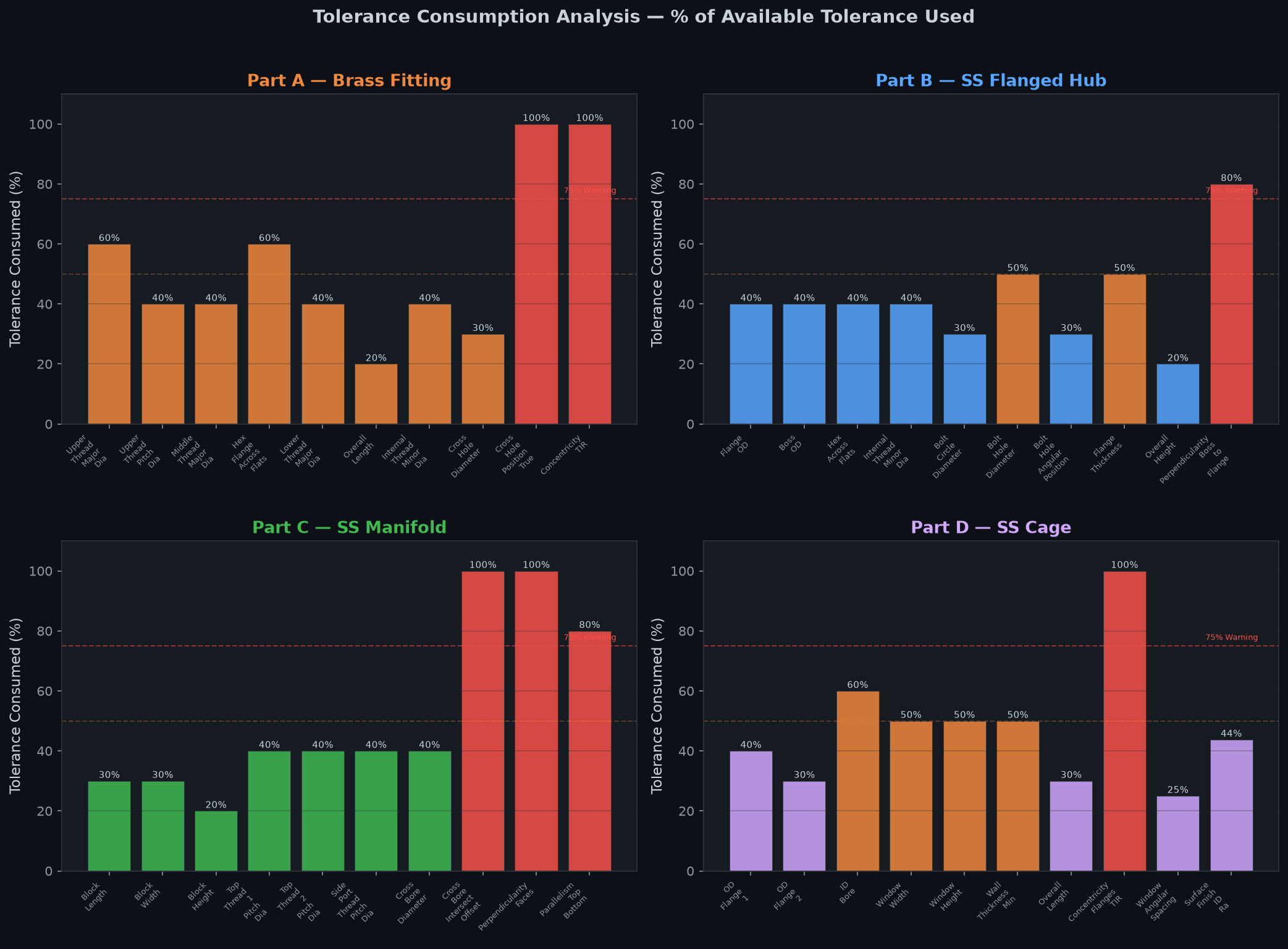
Tolerance stackup analysis — worst-case and RSS (root-sum-square) methods applied to assembly dimension chains.

Tolerance Stack Analysis

Worst-case tolerance consumption analyzed for assembly-critical dimension chains. RSS method applied to multi-feature tolerance stacks to determine statistical assembly clearance.

Understanding tolerance allocation is critical for manufacturing cost optimization — tighter than necessary tolerances add cost without functional benefit.

CNC Machining 5-Axis Metrology / CMM GD&T / ASME Y14.5 SPC / Cpk MAZATROL G-Code GibbsCAM
Project 06

Mortise Lock Reverse Engineering

Full Teardown → CAD Reconstruction → FDM Prototype

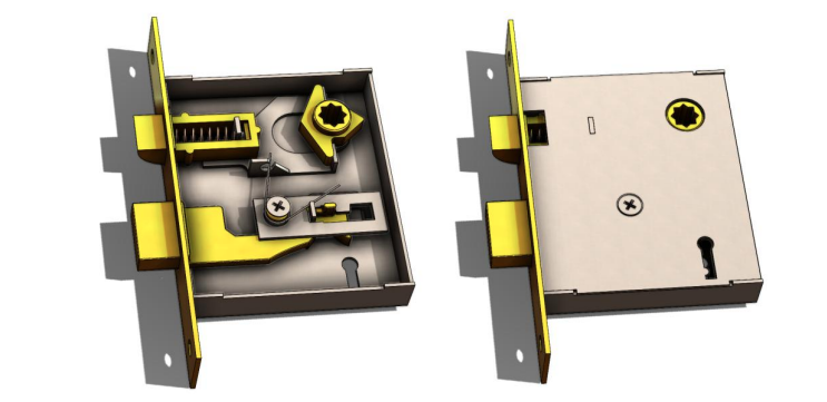
Complete reverse engineering of a commercial mortise lock — from systematic disassembly and precision measurement through parametric SolidWorks reconstruction and functional FDM 3D-printed prototype. A mechanically sophisticated system with ~10 interacting components in a compact volume.

10
Components
10
SLDPRT Files
6
Print Iterations
Functional
Prototype
Assembly & Mechanism
Mortise lock assembly exploded view
Mortise lock SolidWorks assembly — 10 components with full mate relationships enabling kinematic simulation of handle rotation and deadbolt throw.

Reverse Engineering Methodology

6-phase structured workflow: Disassembly → Measurement → CAD Modeling → Assembly → 3D Printing → Functional Validation.

  • Systematic disassembly with component cataloging
  • Digital caliper measurements (0.01mm resolution)
  • Fully parametric SolidWorks models for all 10 components
  • Assembly mates preserving actual kinematics (concentric, coincident, limit mates)
  • FDM 3D printing with tolerance compensation (holes enlarged 0.2–0.4mm)
Engineering Analysis
Spring force curve analysis
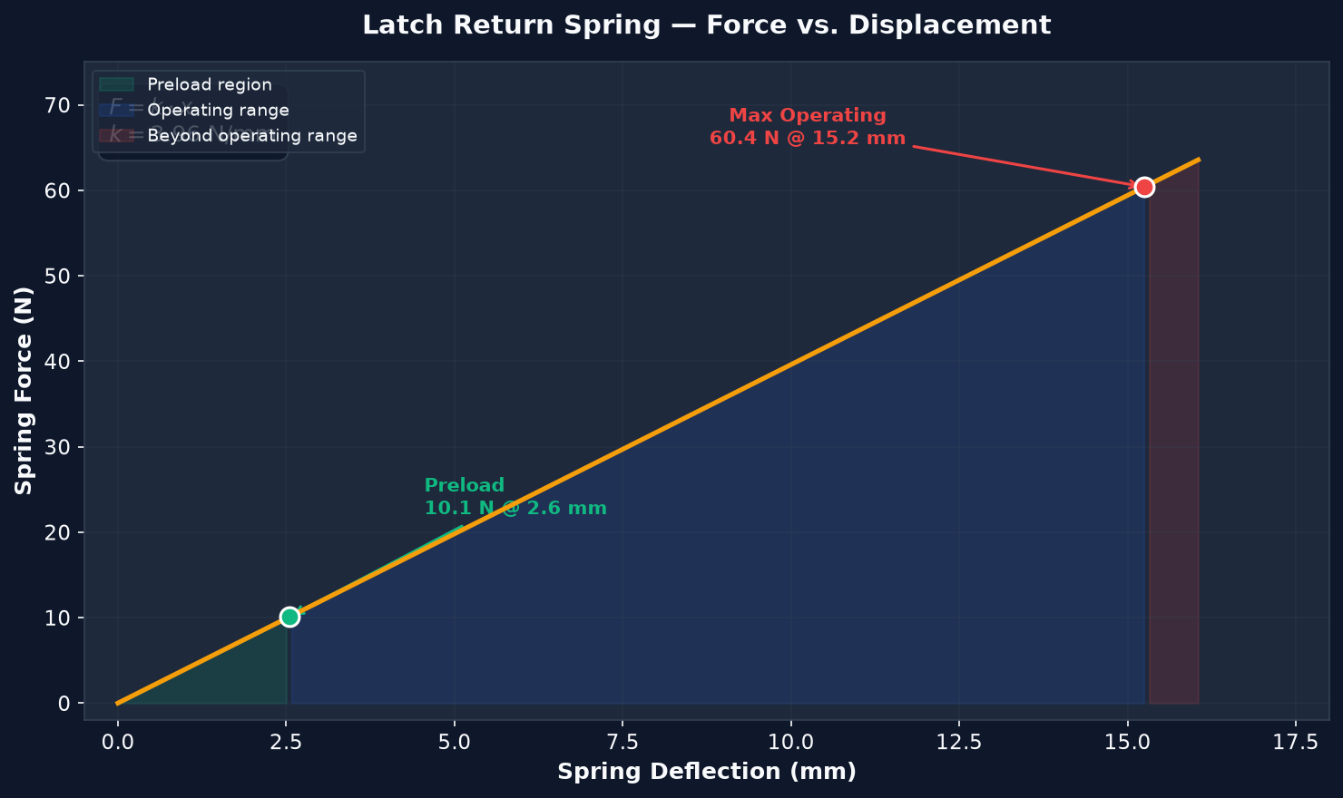
Latch return spring force analysis — Hooke's Law derivation from spring geometry, with Wahl factor correction for shear stress.

Spring & Force Analysis

Derived the spring constant from geometry using the helical compression formula k = Gd&sup4;/(8D³Na) = 3.96 N/mm. Computed preload force (10.10 N) and maximum working force (60.39 N).

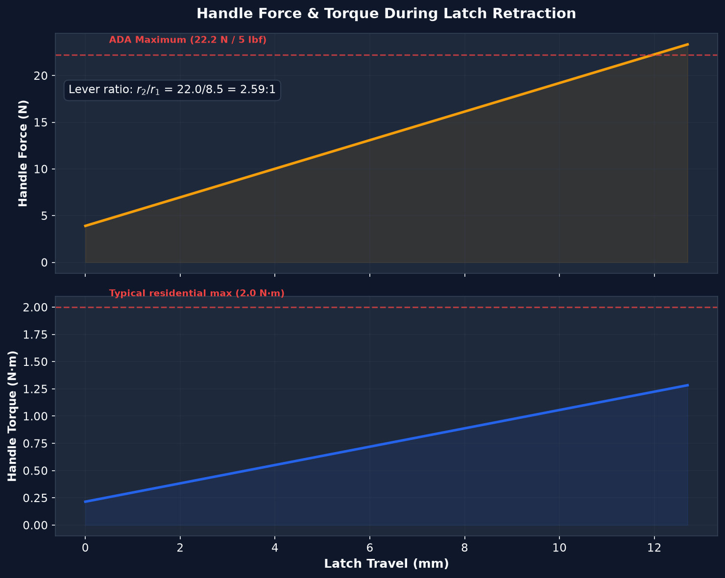
Handle torque for latch retraction: 1.28 N·m — consistent with smooth, comfortable door handle operation.

Cam displacement curve
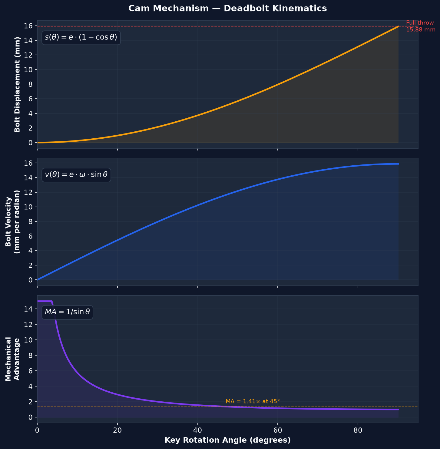
Cam displacement analysis — deadbolt throw (15.88mm) derived from eccentric cam geometry s(θ) = e(1 − cos θ).

Cam Kinematics — Deadbolt Actuation

The deadbolt cam converts ~90° of key rotation into 15.88mm of linear deadbolt travel. The displacement relationship s(θ) = e(1 − cos θ) reveals that mechanical advantage peaks at start (θ → 0) and diminishes as the cam approaches full extension.

Force amplification: MA = 1/sin θ — a 50 N key force generates 70.7 N at the bolt at θ = 45°.

Material comparison — steel vs PLA bolt shear strength
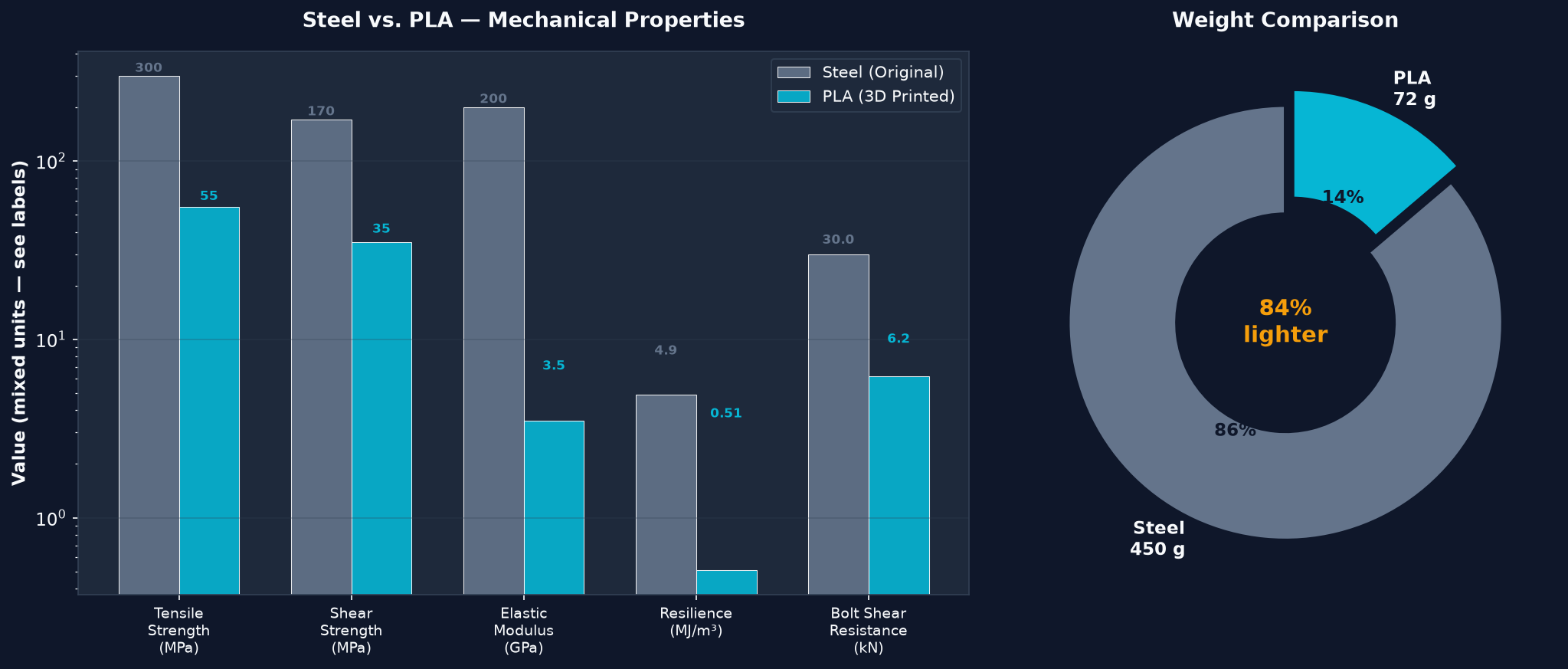
Material substitution analysis — steel bolt (30 kN shear) vs. PLA bolt (6.2 kN shear), PLA provides ~20% of original security but validates mechanism function.

Material Substitution Analysis

Quantified the performance trade-off when substituting PLA for steel:

  • Steel deadbolt shear resistance: 30.0 kN (6,740 lbf)
  • PLA deadbolt shear resistance: 6.2 kN (1,387 lbf)
  • PLA latch bolt bevel angle increased from 15° to 25° to compensate for higher PLA-on-steel friction (μ = 0.35 vs 0.15)

PLA is a functional prototype material — sufficient for mechanism validation but requiring ~20% security margin reduction.

Handle force curve analysis
Handle force requirement curve — lever ratio reduces spring force from 60.39 N to 23.31 N at the handle, confirming comfortable operation.

Handle Ergonomics

The lever mechanism ratio (r1/r2) reduces the spring force experienced at the handle. Maximum handle force of 23.31 N — well below the 50 N threshold for comfortable prolonged operation.

Handle torque: T = F × rhandle = 1.28 N·m — smooth, effortless latch retraction.

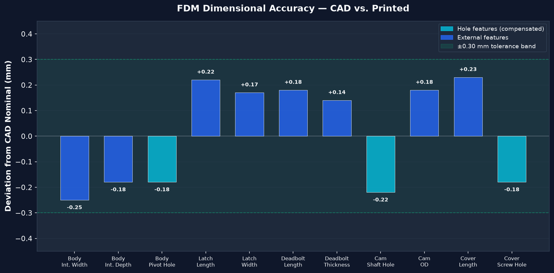
Dimensional deviation — CAD vs physical measurement
Dimensional accuracy analysis — CAD model vs. physical part measurements across all components.

CAD Accuracy Validation

Periodic comparison of CAD geometry against physical parts ensured model accuracy. Design intent preservation: nominal dimensions inferred from measurement clusters, tolerances estimated from measurement scatter.

This process required inferring the designer's intent — not just copying geometry, but understanding why each feature is the size and shape it is.

Reverse Engineering SolidWorks CAD Mechanism Design FDM 3D Printing Cam Kinematics Material Substitution

Engineering Competencies

A cross-section of capabilities demonstrated across six projects — from CNC machining and CAD modeling to embedded systems and machine learning.

Manufacturing & CNC

  • CNC Turning & Milling (3–5 axis)
  • MAZATROL Conversational Programming
  • G-Code (ISO 6983)
  • GibbsCAM Multi-Axis
  • Single-Point Threading
  • Thin-Wall & Multi-Face Machining
  • Blueprint Reading (ASME Y14.5)
📊

Metrology & Quality

  • CMM Operation & Programming
  • GD&T (ASME Y14.5-2018)
  • Process Capability (Cpk/SPC)
  • Surface Profilometry (Mahr MarSurf)
  • Micrometer / Caliper / Pin Gage
  • Thread Gaging (Go/No-Go)
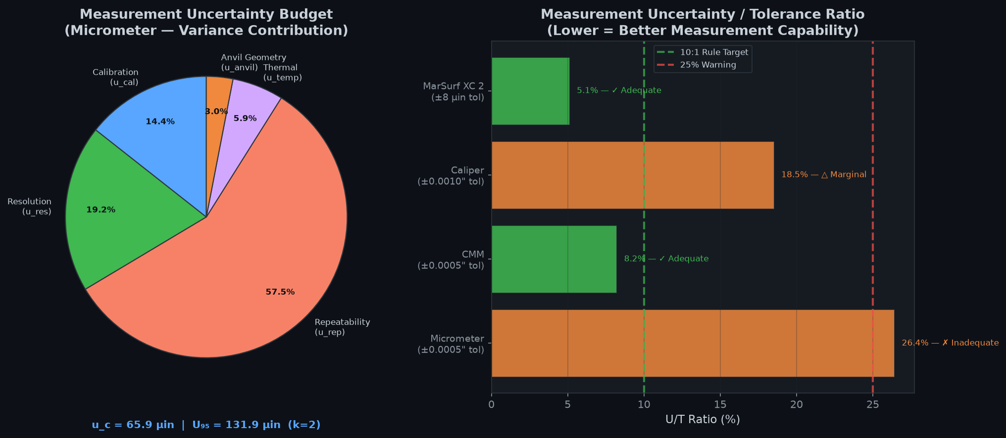
  • Measurement Uncertainty Analysis

CAD & Design

  • SolidWorks Parametric Modeling
  • Part & Assembly Design
  • Reverse Engineering
  • Design for Manufacturability (DFM)
  • Tolerance Stack Analysis
  • GD&T Callouts
  • Engineering Drawings
💻

Controls & Embedded

  • PID Control (Tuning & Implementation)
  • Sensor Fusion (Complementary Filter)
  • Arduino / ATmega328P
  • MATLAB / Simulink
  • Real-Time Embedded Systems
  • Stepper Motor Control (A4988)
  • I2C / SPI / UART Communication
🧮

Analysis & Simulation

  • FEA (Fusion 360)
  • Fluid Dynamics (Bernoulli, Darcy-Weisbach)
  • Structural Analysis (Lamé, Von Mises)
  • Physics-Informed Neural Networks (PINN)
  • Signal Processing (PPG, FFT, Filtering)
  • Statistical Error Analysis
  • FMEA (Failure Mode & Effects)
🔬

Tools & Software

  • Python (PyTorch, NumPy, Matplotlib)
  • SolidWorks + SolidWorks Flow Sim
  • GibbsCAM
  • Git / Version Control
  • Microsoft Excel (Data Analysis)
  • Arduino IDE
  • Fusion 360 (CAD + FEA)